This Artifacts Log post is unusual in how many diverse, quirky models there are across use-cases and modalities. Normally these model roundups are dominated by big models from the likes of Qwen, DeepSeek, Kimi, etc. There are models for all sorts of different use-cases in this post, from optical character recognition (OCR), RAG search, audio transcription, computer-use, code-editing, math theorem proving, and more. The artifacts covered this month also come from a much broader list of open model builders.
This gives us a lot of hope for the future of open models, where we see the need for domain-specific, cheap models as being crucial tools to complement the strongest, closed agents. When the top few models get the headlines, this vast, industry-scale tinkering can easily be forgotten. Reading this post gives a technically grounded, broad coverage of the many directions the industry is pushing specific models for. Expect more like this!
To encourage people to take a look at the diversity of models in this issue, the core part of the update is not paywalled. An otherwise quiet month at the top end of open models really delivered.
Artifacts Log
Our Picks
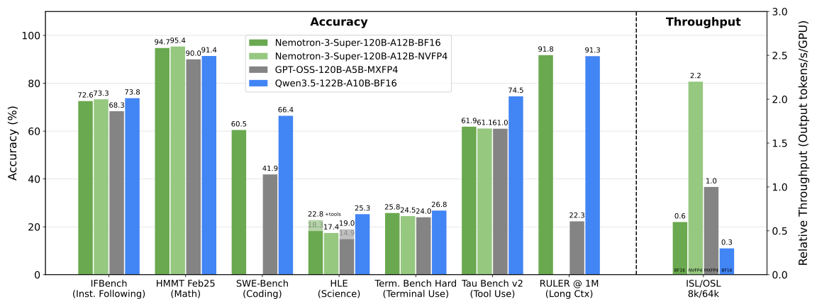
NVIDIA-Nemotron-3-Super-120B-A12B-NVFP4 by nvidia: The long-awaited mid-sized model from NVIDIA is finally here: 120B total params with 12B active, a 1M context window, and support for multiple popular languages. Furthermore, the model is based on LatentMoE and uses NVFP4 during pre-training, which is a first for open models. Like other things from NVIDIA, it comes with an in-depth tech report plus pre-training and post-training datasets, with the vast majority of the data being openly released.
cohere-transcribe-03-2026 by CohereLabs: A speech-to-text model by Cohere based on the conformer architecture, similar to NVIDIA’s Parakeet. It features 14 different languages, including some AIPAC languages and Arabic. Performance-wise, Cohere claims it beats similarly sized open and closed models. To top it all off: The model is released under Apache 2.0! Previous open models by Cohere were released under a non-commercial license.
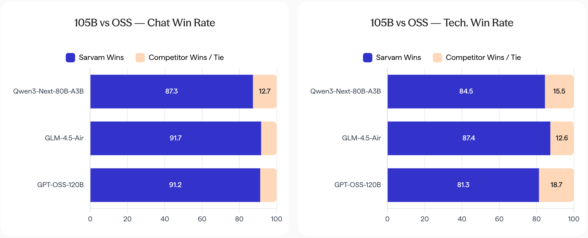
sarvam-105b by sarvamai: The Indian startup Sarvam, which trained open models in the past, has scaled up everything for its new flagship models in terms of dataset size (12-16T tokens) and model size (30B-A2B, 105B-10A). As a result, they come close to or even surpass a lot of open models with similar sizes. The release also shows why sovereign AI is so important, something that few other countries have internalized yet: In comparison with SOTA open models, the Sarvam models are vastly more preferred in Indic languages.
Mistral-Small-4-119B-2603 by mistralai: A 119B-A7B model by Mistral, combining their previous model generations into one as a hybrid reasoning model with coding abilities.
zeta-2 by zed-industries: The open source code editor Zed has released their edit prediction model openly in the past, which we featured a year ago. While the previous version was based on open data, the new version, based on Seed-Coder-8B, is trained on open source code by users who explicitly opted into data collection.
Models
General Purpose
gpt-oss-puzzle-88B by nvidia: A pruned expert version of GPT OSS 120B. It also replaces some global attention layers with window attention. Puzzle is “a post-training neural architecture search (NAS) framework, with the goal of significantly improving inference efficiency for reasoning-heavy workloads while maintaining or improving accuracy across reasoning budgets.”
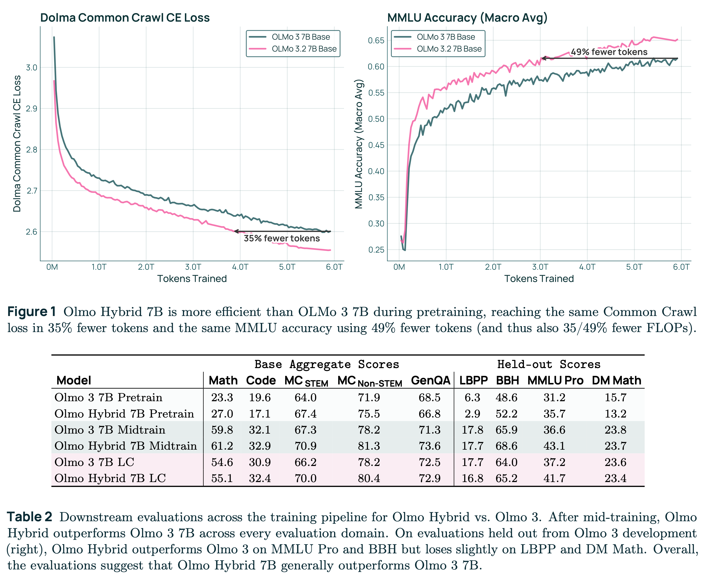
Olmo-Hybrid-7B by allenai: A hybrid attention + GDN (gated DeltaNet) model. See our blog post for more insights about the architecture and its challenges.
NVIDIA-Nemotron-3-Nano-4B-BF16 by nvidia: A compressed version of NVIDIA-Nemotron-Nano-9B-v2, which itself is a compressed version of NVIDIA-Nemotron-Nano-12B-v2. Nvidia has been pushing this direction more than anyone else with open models.
Multimodal
Yuan3.0-Ultra by YuanLabAI: A 1T multimodal model by the relatively unknown Yuan Lab. They pre-trained a 1.5T model on 2.2T tokens and subsequently pruned experts with a new technique, outlined in the tech report.
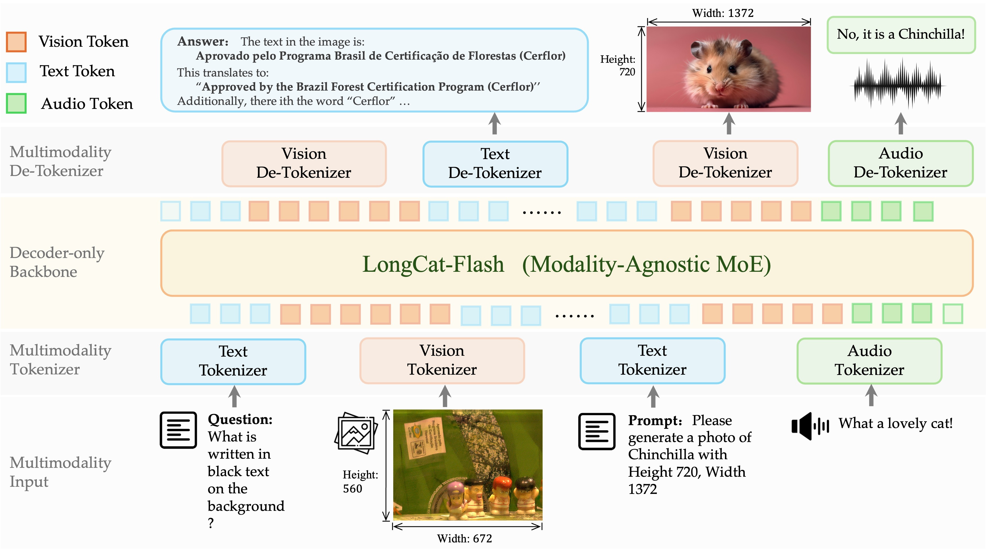
LongCat-Next by meituan-longcat: A multimodal model which can process text, vision, and audio as both inputs and outputs.
granite-4.0-1b-speech by ibm-granite: A small speech-to-text model supporting six languages. It also supports the generation of English audio for translation.
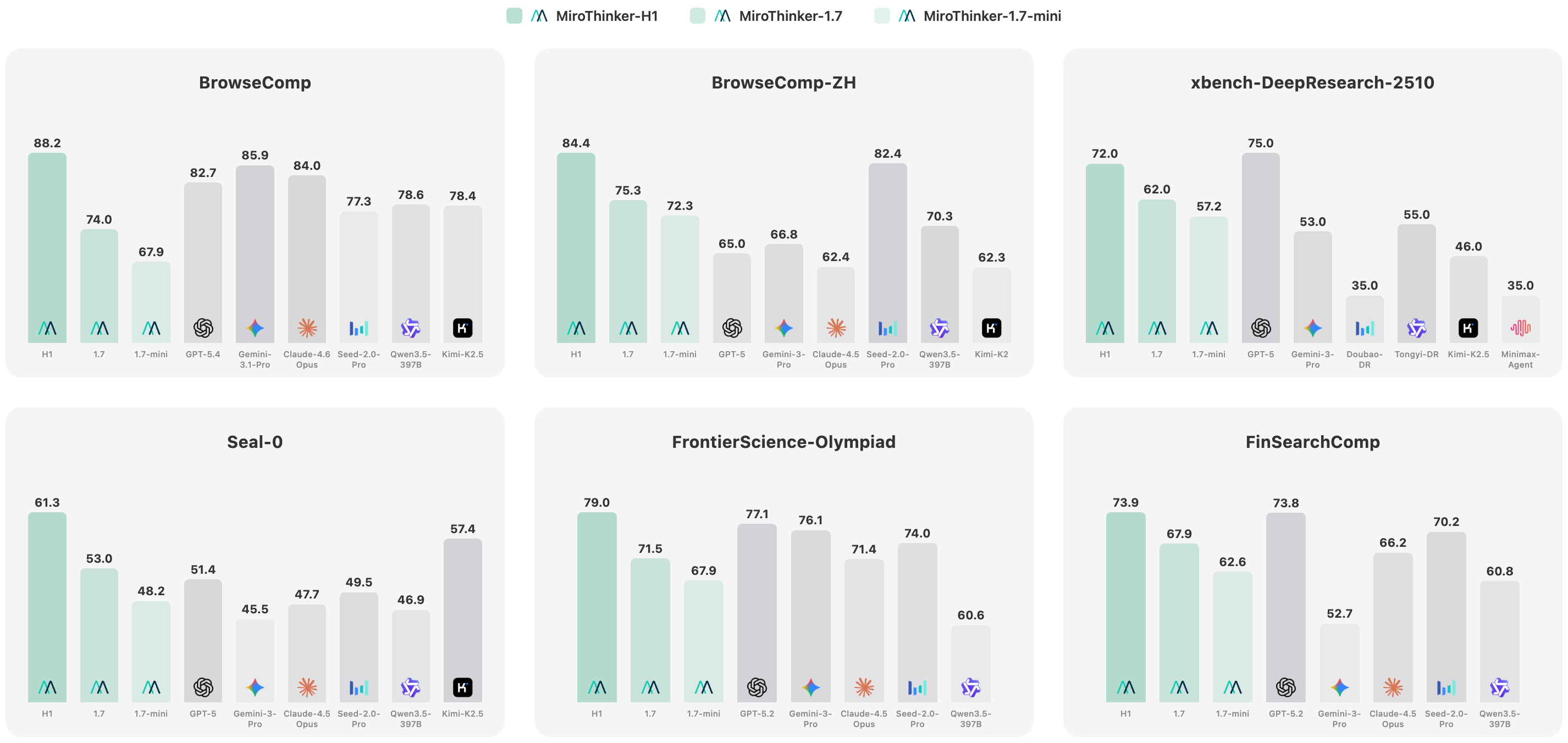
MiroThinker-1.7 by miromind-ai: A fine-tuned version of Qwen 235B for agentic workflows, especially research.
tabpfn_2_6 by Prior-Labs: An update to the popular tabular prediction model, which is slightly larger than its predecessor. Its license allows research and internal evaluation only.
sam3.1 by facebook: An update to SAM 3, carrying the same restrictive license.
reka-edge-2603 by RekaAI: A model for robotics, beating models such as Cosmos-Reason2. Its noncommercial license converts into Apache 2.0 after two years.
RAG
Qianfan-OCR by baidu: There have been a lot of great OCR models lately. This one is from Baidu and is licensed under Apache 2.0.
chandra-ocr-2 by datalab-to: An update to the Chandra OCR model, released under a restrictive license.
Reason-ModernColBERT by lightonai: A SOTA retrieval model released under a non-commercial license. However, there is also code to re-generate the data, allowing the training of a commercially viable version.
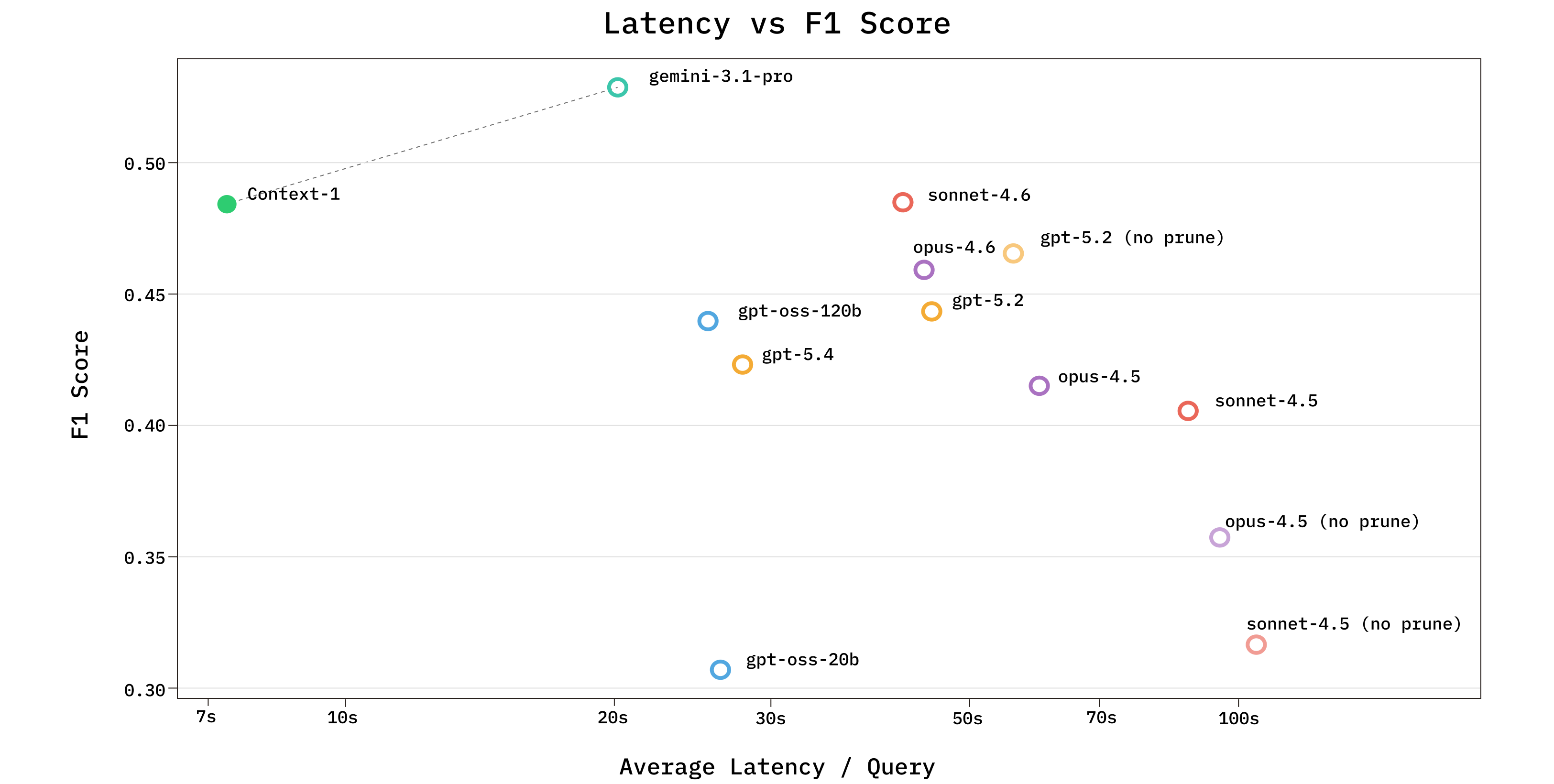
context-1 by chromadb: A fine-tuned version of GPT-OSS for agentic search with an in-depth tech report. It also marks the debut of Chroma into the open model space. Trained with Thinking Machine’s Tinker.
dots.mocr by rednote-hilab: The beloved dots.ocr model has been updated and supports SVG outputs. However, on top of the general MIT license, the model comes with additional usage restrictions, just like its predecessor.
Learn how OpenAI’s Model Spec serves as a public framework for model behavior, balancing safety, user freedom, and accountability as AI systems advance.
OpenAI launches a Safety Bug Bounty program to identify AI abuse and safety risks, including agentic vulnerabilities, prompt injection, and data exfiltration.
Participatory AI initiatives are meant to bring together diverse stakeholders to design and oversee AI systems that are fair and trustworthy. However, a recent review of 80 participatory AI initiatives revealed that, rather than providing participants with genuine decision-making power, the vast majority consult specific communities on narrow implementation details.
Meanwhile, every major AI lab now conducts some form of public consultation, the EU AI Act requires stakeholder involvement, and the OECD AI Principles regard stakeholder engagement as a fundamental element of trustworthy AI. Participation in AI governance has become more popular than ever. But an uncomfortable pattern is emerging: the more we discuss participation, the less we discuss meaningful engagement, real influence and power.
Many participatory approaches primarily involve communities during the early stages of the AI system lifecycle: design, data collection, and model development, while later stages, such as deployment, monitoring and system evolution, attract far less attention. During my fieldwork across Kenya, Malawi, and the Philippines, a troubling question keeps surfacing: once the participatory design phase concludes, who truly governs the AI system? Even highly participatory processes often dissolve once the system is launched. Governance then shifts back to those who built or commissioned the system. Communities involved in shaping the design often have little influence over how systems evolve to meet ongoing community needs or how they expand beyond their initial scope.
The old lesson we keep relearning
Back in 1969, urban planner Sherry Arnstein published a deceptively simple insight: not all participation redistributes power. Her “ladder of citizen participation” described eight levels, from manipulation at the bottom to citizen control at the top. She called the middle rungs “tokenism”: processes that perform inclusion without actually transferring authority. Arnstein was writing about urban planning in American cities, but her framework resonates powerfully in today’s AI landscape.
Over fifty years later, AI researchers are revisiting this lesson. Recent studies have introduced the concept of “participation washing”: the act of claiming inclusion without the necessary redistribution of power. Other researchers have documented how participatory rhetoric often conceals the ongoing centralisation of decision-making authority.
These findings paint a consistent picture. Participatory AI, despite methodological progress, largely remains at Arnstein’s “consultation” and “informing” levels rather than reaching the “partnership” or “delegated power” levels. The reasons for this are understandable. Genuine participation is costly, slow, and fosters accountability relationships that complicate rapid development and deployment cycles. Organisations optimising for scale naturally minimise governance complexity. However, this means participatory AI often reproduces the very power imbalances it seeks to address.
Sherry Arnstein’s ladder of citizen participation
The real divide: Methods versus infrastructure
Despite all this, the field has made genuine progress in developing methods to meaningfully involve people in AI design. The repository of tools and metrics on the OECD.AI Policy Observatory showcases participatory frameworks that now guide humanitarian and public sector AI initiatives globally. Methods have become increasingly sophisticated, moving beyond superficial consultation towards authentic co-design. What remains underdeveloped is the infrastructure for ongoing governance after deployment.
Think of it this way. Methods answer: “How do we involve people in design?” Infrastructure addresses: “How do people exercise authority after deployment?”
This distinction matters because AI systems, as the OECD definition emphasises, are adaptive. They are never “finished.” They evolve continuously through new training data, model updates, and deployment expansions. Each evolution requires governance decisions.
AI also relies on collective data. These are not tools that individuals choose to use; rather, they are infrastructure that processes communal information and makes decisions that affect entire populations. Without proper governance, participation during the design phase can inadvertently legitimise systems that centralise power. “We consulted the community” becomes a justification for deployment, even if communities no longer hold any authority over the system’s future.
What commons governance looks like in practice
If the challenge is institutional, what institutional forms could address it? One promising approach draws on principles from natural resource commons. Economist Elinor Ostrom received the Nobel Prize for demonstrating that communities can effectively manage shared resources such as fisheries, forests and irrigation systems. The application of commons governance to knowledge and digital resources has been extensively developed in later work, from Hess and Ostrom’s study of knowledge commons to comprehensive frameworks for analysing knowledge commons governance across various institutional contexts.
Commons governance models have several features that matter for AI: collective ownership, where communities hold rights to the resource; participatory decision making, where rules for usage and development are established through community processes; value sharing, where benefits are returned to the community; and continuous stewardship, where governance continues as long as the system operates.
The work I contribute to involves exploring whether these principles can guide AI system development in resource-limited settings. In Malawi, our research team at NYU and our local partners are creating a voice-based crisis reporting system designed to ensure that community governance councils oversee data practices, model updates, and deployment decisions. In the Philippines, we are collaborating with Kalinga State University on an Indigenous Knowledge Data Collaborative that allows communities to control how their traditional knowledge is digitised and used. The CARE Principles for Indigenous Data Governance, emphasising Collective benefit, Authority to control, Responsibility, and Ethics, offer a powerful framework here. These principles emerged from broader movements around Indigenous data sovereignty and represent a significant way to reshape data governance around community authority rather than external oversight.
While the OECD AI Principles mention data trusts as a mechanism for ethical data sharing, commons models take this logic further. Data trusts typically delegate authority to trustees acting on a community’s behalf. Commons models place community decision-making at the centre. The community does not transfer control to a benevolent intermediary; it retains authority itself.
Initiatives like Mozilla Common Voice and various Indigenous data-sovereignty movements are exploring this path worldwide, yet critical questions persist. Can commons governance operate effectively in resource-limited humanitarian settings? What occurs when commons governance moves too slowly for operational needs? Our fieldwork aims to address these exact questions.
What we are learning and what presents challenges
I want to be frank about the limitations of this work. These are early-stage experiments, not established models. However, they reveal important tensions that the wider field needs to address. If participatory AI governance is to go beyond words, we must be honest about what makes it challenging.
Power redistribution is costly. Governance meetings involve travel expenses, translation services, and participant compensation. In our work in Malawi, these costs are significant and surpass typical AI development budgets. However, this should be viewed not just as an expense but as an investment in risk mitigation. Without this investment, systems in complex environments risk rejection, non-adoption and even obsolescence.
Democracy is slow, and crises are urgent. Emergency responses demand quick decisions. Community governance takes time. The challenge is to differentiate between decisions that truly require rapid centralised action and those that only seem urgent to technical implementers.
“Community” is not uniform. Gender, age, and ethnicity influence who takes part and whose voice carries weight, and commons governance does not automatically resolve representation issues. However, it does make them visible and demands specific mechanisms to address them.
Sustainability remains uncertain because meaningful participation requires ongoing resources; governance cannot be an afterthought funded by short-term grants. It must be incorporated into budgets from the outset and treated as operational expenditure. International development finance models will need to adapt to support this. A system that works brilliantly for two years and then collapses because governance funding runs out is not a success.
What this means for AI policy
These experiments demonstrate methods to strengthen international frameworks for stakeholder engagement.
First, we need clearer distinctions between engagement levels. Consultative engagement involves gathering input to inform others’ decisions. Governance authority means stakeholders exercise binding power over system operation. Frameworks often conflate these two very different concepts. When a government or company says it has “engaged stakeholders,” does that mean it sought feedback or that it shared power? Making this distinction explicit helps implementers understand what they are truly committing to, and helps communities know what to expect.
Second, resource models need to change. Governance infrastructure, including ongoing meetings, capacity building, and conflict resolution, should be seen as a way to protect assets rather than as overhead. Current assessments of AI pilots rarely differentiate between technical and governance factors when a project fails. This complicates the process of allocating resources effectively. Funding structures must recognise that governance is the mechanism that maintains an AI system’s viability and trust over time.
Third, we need governance metrics. The OECD effectively monitors AI policy implementation. But we also need ways to measure the quality of power distribution. Who makes binding decisions about how a system evolves? Just as “technical debt” builds up when code is rushed, “governance debt” accumulates when engagement is overlooked. Eventually, the interest is paid in the form of lost trust or system failure. Recent work on AI accountability frameworks suggests promising directions for creating such assessments.
Finally, community data ownership has an unclear legal status in most jurisdictions. Cross-jurisdictional research on legal frameworks that support collective governance would be very valuable. Experiments such as New Zealand’s Māori data sovereignty frameworks and Barcelona’s data cooperatives offer promising models to learn from. The goal is not to impose universal frameworks but to document what works, what does not, and where the legal gaps are most severe.
Community governance authority as infrastructure
The participatory turn in AI governance represents genuine progress. However, involving people during design without engaging them in governance risks becoming a sophisticated form of consultation that maintains existing power structures. This is exactly what Arnstein warned against more than fifty years ago.
Moving from participation to power involves treating community governance authority as infrastructure: something that requires investment, upkeep, and institutional backing comparable to the technical systems it oversees. It means funding that supports governance alongside technical development. It means metrics that evaluate power distribution, not just engagement processes. And it means honest recognition that meaningful participation is slower and more costly than consultation, but also more likely to produce systems that communities genuinely trust and use over the long term.
Eighty participatory AI initiatives were reviewed, and most of them never moved beyond consultation. That finding should concern anyone who values participation. If we are serious about closing the gap between engagement and authority, we must start building the governance infrastructures to do it. AI remains in its early stages, and there is much we still need to understand. But one thing is becoming clear: if AI is considered infrastructure, it requires governance infrastructure. Otherwise, there is no trustworthy AI.
The international community has made significant progress in defining what responsible AI looks like. The next step is investing in the unglamorous, difficult, and necessary work of establishing governance structures to uphold these standards. This involves supporting communities not only as participants in design but also as equal partners in decision-making.
Fast takeoff, the singularity, and recursive self-improvement (RSI) are all top of mind in AI circles these days. There are elements of truth to them in what’s happening in the AI industry. Two, maybe three, labs are consolidating as an oligopoly with access to the best AI models (and the resources to build the next ones). The AI tools of today are abruptly transforming engineering and research jobs.
AI research is becoming much easier in many ways. The technical problems that need to be solved to scale training large language models even further are formidable. Super-human coding assistants making these approachable is breaking a lot of former claims of what building these things entailed. Together this is setting us up for a year (or more) of rapid progress at the cutting edge of AI.
We’re also at a time where language models are already extremely good. They’re in fact good enough for plenty of extremely valuable knowledge-work tasks. Language models taking another big step is hard to imagine — it’s unclear which tasks they’re going to master this year outside of code and CLI-based computer-use. There will be some new ones! These capabilities unlock new styles of working that’ll send more ripples through the economy.
These dramatic changes almost make it seem like a foregone conclusion that language models can then just keep accelerating progress on their own. The popular language for this is a recursive self-improvement loop. Early writing on the topic dates back to the 2000s, such as the blog post entirely on the topic from 2008:
Recursion is the sort of thing that happens when you hand the AI the object-level problem of “redesign your own cognitive algorithms”.
A seed AI is an AI designed for self-understanding, self-modification, and recursive self-improvement. This has implications both for the functional architectures needed to achieve primitive intelligence, and for the later development of the AI if and when its holonic self-understanding begins to improve. Seed AI is not a workaround that avoids the challenge of general intelligence by bootstrapping from an unintelligent core; seed AI only begins to yield benefits once there is some degree of available intelligence to be utilized. The later consequences of seed AI (such as true recursive self-improvement) only show up after the AI has achieved significant holonic understanding and general intelligence.
It’s reasonable to think we’re at the start here, with how general and useful today’s models are.
Generally, RSI can be summarized as when AI can improve itself, the improved version can improve even more efficiently, creating a closed amplification loop that leads to an intelligence explosion, often referred to as the singularity. There are a few assumptions in this. For RSI to occur, it needs to be that:
The loop is closed. Models can keep improving on themselves and beget more models.
The loop is self-amplifying. The next models will yield even bigger improvements than the current ones.
The loop continues to run without losing efficiency. There are not added pieces of friction that make the exponential knee-capped as an early sigmoid.
While I agree that momentous, socially destabilizing changes are coming in the next few years from sustained AI improvements, I expect the trend line of progress to be more linear than exponential when we reflect back. Instead of recursive self-improvement, it will be lossy self-improvement (LSI) – the models become core to the development loop but friction breaks down all the core assumptions of RSI. The more compute and agents you throw at a problem, the more loss and repetition shows up.
Interconnects AI is a reader-supported publication. Consider becoming a subscriber.
I’m still a believer that the complexity brake on advanced systems will be a strong counterbalance to the reality that AI models are getting substantially better at every narrow task we need to compose together in making a leading AI model. I quoted this previously in April of 2025 in response to AI 2027.
Microsoft co-founder Paul Allen argued the opposite of accelerating returns, the complexity brake: the more progress science makes towards understanding intelligence, the more difficult it becomes to make additional progress. A study of the number of patents shows that human creativity does not show accelerating returns, but in fact, as suggested by Joseph Tainter in his The Collapse of Complex Societies, a law of diminishing returns. The number of patents per thousand peaked in the period from 1850 to 1900, and has been declining since. The growth of complexity eventually becomes self-limiting, and leads to a widespread “general systems collapse”.
There are plenty of examples in how models are already trained, the deep intuitions we need to get them right, and the organizations that build them that show where the losses will come from. Building leading language models is incredibly complex, and only becoming more-so. There are a few core frictions in my mind.
1. Automatable research is too narrow
First, it is clear that language models this year will already be useful tools at optimizing localized tasks like lowering the test loss of a model. Andrey Karpathy recently launched his autoresearch that popularized doing just this. This allows AI agents to play directly on GPUs to target tasks like lowering the loss on the test set. This approach works in narrow domains, i.e. one general test loss or one overall reward. The problem is that there’s a long-standing gap between an on-paper more accurate model and models that users find more productive. The most provocative case is for pretraining, which was discussed more at length around scaling laws. Scaling laws show us that the loss will continue going down, but we don’t know if that’ll be economically more valuable.
In post-training, reinforcement learning algorithms are at least more directly tied to specific performance gains as most RL training environments can be used directly as an evaluation. Still, I worry about generalization and tying back to models that are better at the specific task of improving themselves. It’s a big leap from models get better at some things to that necessarily translating to models that are better at building themselves and designing experiments. We’ve seen many AI capabilities sort of saturate at certain levels of human taste, such as writing quality. AI research is a bit different here, as there is a very high ceiling to climb up to. Where models mostly saturate on writing because there’s inherent tension in preferences, models will saturate on research because the search space and optimization target is too wide.
The early benchmarks for measuring this sort of ability all fall prey to the same problem – narrow scope. Agents will do well at optimizing single metrics, but the leap required to navigate many metrics at once is a very different skill set. That is actually what the best researchers do — they make many scalable ideas work together.
The most related benchmark we have to measure this is PostTrainBench, which is quite fun, but progress will very rapidly get distorted on this. Over 90% of the challenge in doing post-training well is getting the last 1-3% of performance, especially without cooking the model in out-of-domain tasks. Post-training a general, leading model is extremely complex, and only getting more complex.
I could go on and on about this. Another example is from during my Ph.D. (2017-2022), when there was immense hype around a field called “AutoML” which aimed to use techniques like Bayesian Optimization to find new architectures and parameters for models. The hype never translated into changing my job. Language models will do more than this, but not enough to take jobs away from top AI researchers any time soon. The core currency of researchers is still intuition and managing complexity, rather than specific optimization and implementation.
2. Diminishing returns of more AI agents in parallel
The biggest problem for rapid improvement in AI is that even though we’ll have 10,000 remote workers in a datacenter, it’ll be nearly impossible to channel all of them at one problem. Inherently, especially when the models are still so similar, they’re sampling from the same distribution of solutions and capabilities while being bottlenecked by human supervision. Adding more agents will have a strict saturation in the amount of marginal performance that can be added – the intuition of the best few researchers (and time to run experiments) will be the final bottleneck.
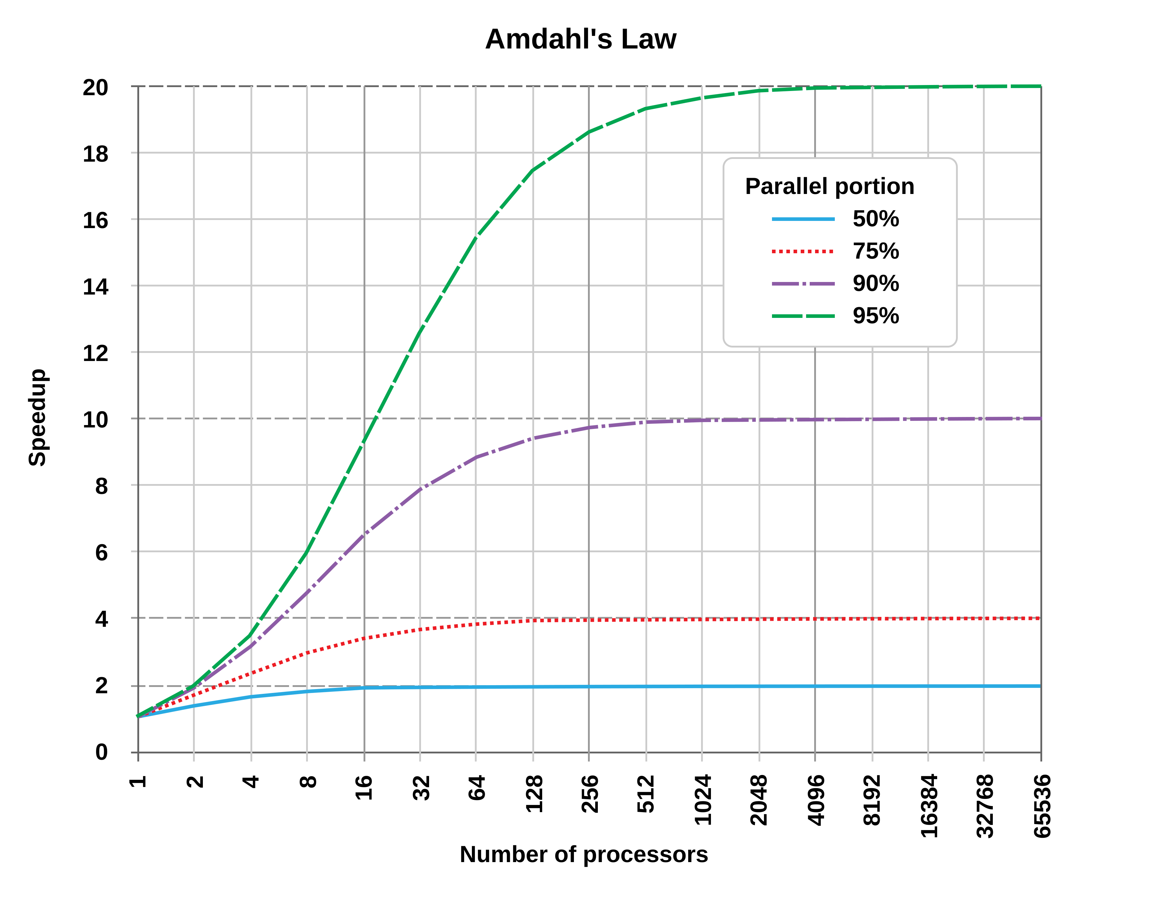
A common idea to illustrate this is Amdahl’s law, which is taken from computer architecture and shows that a given task can only generate a fixed speedup proportional to how much can be parallelized and how many parallel workers exist. An illustration is below:
In AI this should be relatively easier to convey, as the low-level operating details of computers are fairly mysterious. Consider an AI researcher on the transition from writing code by hand to using AI autocomplete assistance to now using autonomous coding agents. These are all massive gains. Let us continue. Now this researcher uses 3-4 agents working on different sub-tasks or approaches to the problem at hand. This is still a large gain. Now consider this single researcher trying to organize 30-40 agents with tasks to do every day. Some people can get more value out of this scale, but not many.
How many people do you think could come up with 300-400 tasks for AI agents every day? Not many. This problem will hit the AI models soon enough as well.
3. Resource bottlenecks and politics
Fundamentally, all the AI companies are walking a fine line of acquiring substantial capital, converting new compute resources to revenue via sufficient demand, and repeating the process all-the-while spending an extreme amount on research. With the scale of resources here, there will always be political bottlenecks on who gets resources and what gets bet on. In this layer, research leadership sits above the AIs and the researchers. Even as models continue to improve, this source of friction will never get removed. It isn’t a substantial friction, but the AI models are fundamentally operating in organizations where humans are the bottleneck on resources.
The early scale of improvements with language models is local optimizations, where the resources used cost <$1M per day. With my other views on the frictions of AI, this is on its own a very minor impact on the rate of improvement, but for those with worries of fast take-off, RSI, and loss of control to AIs, it should be obvious that billions of dollars of compute resources for research are unlikely to be totally isolated for end-to-end experimentation of AI models.
The conclusion here is that because we’re at the early stages of using AI assistance, autonomously and at scale for AI-development, we’re collectively discovering the ways that AI can help us massively. We’re all applying these tools to capture the low-hanging fruit we see and our jobs are literally changing to be higher paced and more productive. The problem is that all of these axes have clear human, political, or technical complexity bottlenecks.
The bottom of every sigmoid feels like an exponential. We’ve ridden multiple exponentials in the era of language models, in 2023 we scaled to huge models and GPT-4 felt like magic, by 2025 we added inference-time scaling with o1 and reasoning models — they let us “solve” math and coding, now we’re going to take a big step by polishing the entire AI workflow (all the while scaling training compute massively). 2026 will feel like a huge step, but it doesn’t have a fundamental change convincing me that progress will begin to take off.
This could still cross the colloquial threshold for AGI, which is a drop-in replacement for most remote workers, which would be an incredible milestone. Much of the challenge in the debate of if we hit AGI in the coming years is that AI models are jagged and smart in different ways than humans, so they won’t look like drop-in replacements for remote workers, but in many cases just using AI will be far more effective than trying to work with a human. It’s reshaping what jobs are.
Let us consider the scenarios we’re working through.
Engineering is becoming automated today. Humans are way more productive, models can scale through complex infrastructure deployments much faster, run with higher GPU utilization, etc. Infrastructure gains become fixed improvements in the rate and scale of experimentation, the fundamental units of progress in AI.
Basic AI model research and optimization will be automated. The AI models are expanding in scope – they transition from writing kernels to deciding on architectures. This is moving from improving the experimentation toolkit to running minor experiments themselves. Configs, hyperparameters, etc. become the domain of the AI assistants.
These are both real. The problem is that a third era doesn’t have a simple scale to jump to. Where the AI models can create knowledge by synthesis and execution, the next jump requires harnessing thousands of agents or having models make more novel discoveries – like unlocking the next paradigm after inference time scaling. The improvements downstream of AI are going to make the industry supercharged at hill climbing, but I worry that this won’t bring paradigm shifts that are needed for new categories of AI – continual learning, world models, whatever your drug of choice is.
All together, the models are becoming core to the development loop and that’s worth being excited (and worried) about. The models are performing self-improvement. They’re not transforming the approach. We are scaling up the compute we spend on our own research practices and tools. There are diminishing returns. Agents are going to start being autonomous entities we work with. They feel like a cross between a genius and a 5 year old. We will be in this era of lossy self-improvement (LSI) for a few years, but it is not enough for a fast takeoff.
I had originally planned to write about DeepSeek V4. Since it still hasn’t been released, I used the time to work on something that had been on my list for a while, namely, collecting, organizing, and refining the different LLM architectures I have covered over the past few years.
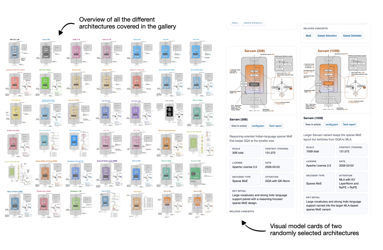
So, over the last two weeks, I turned that effort into an LLM architecture gallery (with 45 entries at the time of this writing), which combines material from earlier articles with several important architectures I had not documented yet. Each entry comes with a visual model card, and I plan to keep the gallery updated regularly.
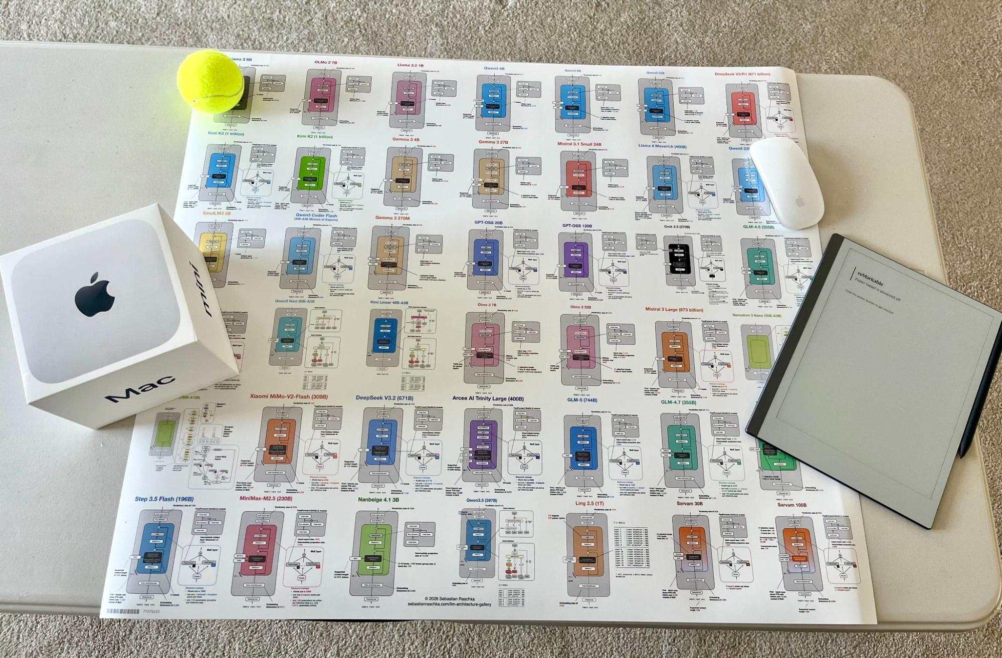
After I shared the initial version, a few readers also asked whether there would be a poster version. So, there is now a poster version via Redbubble. I ordered the Medium size (26.9 x 23.4 in) to check how it looks in print, and the result is sharp and clear. That said, some of the smallest text elements are already quite small at that size, so I would not recommend the smaller versions if you intend to have everything readable.
Figure 2: Poster version of the architecture gallery with some random objects for scale.
Alongside the gallery, I was/am also working on short explainers for a few core LLM concepts.
So, in this article, I thought it would be interesting to recap all the recent attention variants that have been developed and used in prominent open-weight architectures in recent years.
My goal is to make the collection useful both as a reference and as a lightweight learning resource. I hope you find it useful and educational!
1. Multi-Head Attention (MHA)
Self-attention lets each token look at the other visible tokens in the sequence, assign them weights, and use those weights to build a new context-aware representation of the input.
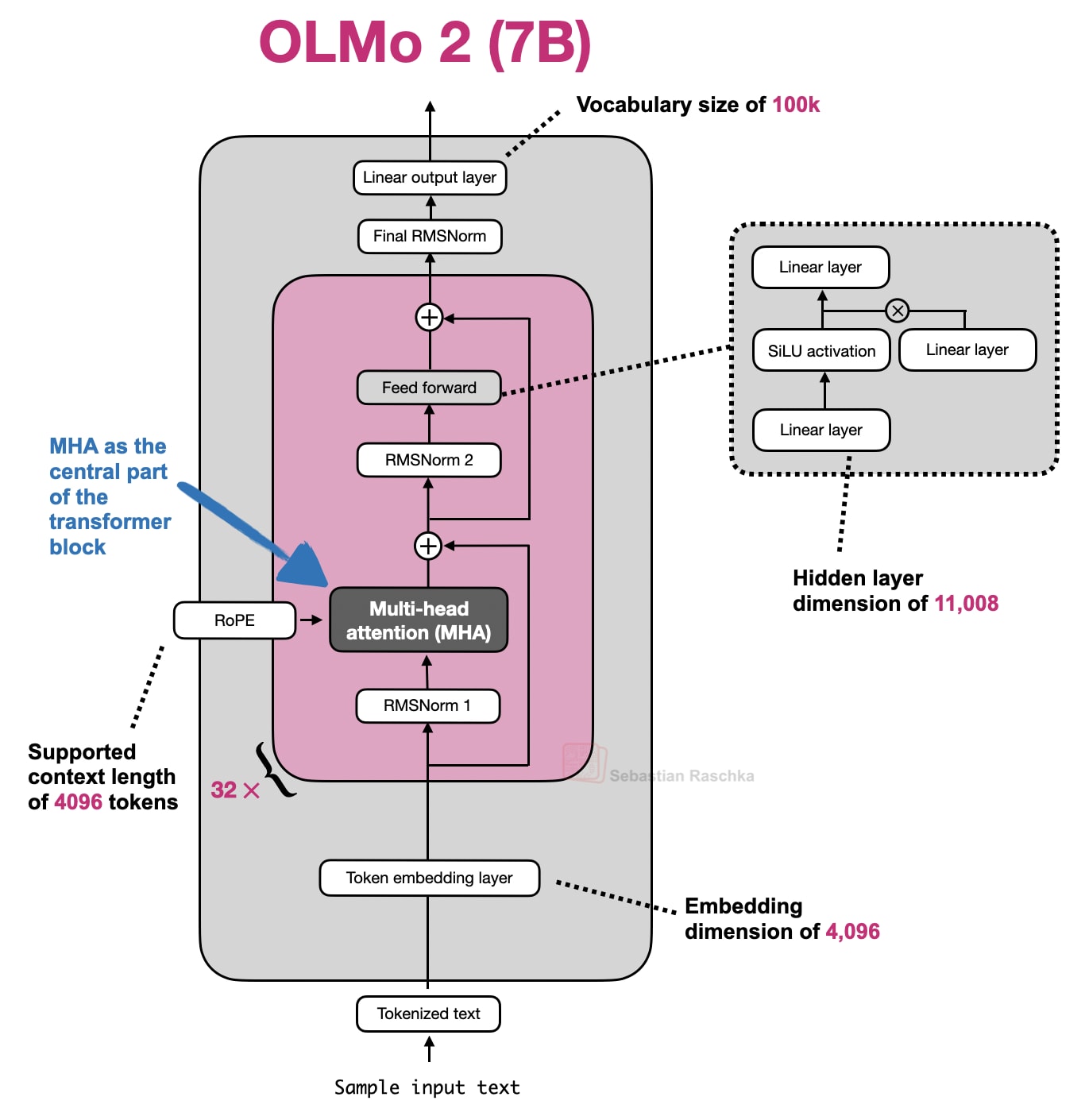
Multi-head attention (MHA) is the standard transformer version of that idea. It runs several self-attention heads in parallel with different learned projections, then combines their outputs into one richer representation.
Figure 3: Olmo 2 as an example architecture using MHA.
The sections below start with a whirlwind tour of explaining self-attention to explain MHA. It’s more meant as a quick overview to set the stage for related attention concepts like grouped-query attention, sliding window attention, and so on. If you are interested in a longer, more detailed self-attention coverage, you might like my longer Understanding and Coding Self-Attention, Multi-Head Attention, Causal-Attention, and Cross-Attention in LLMs article.
1.2 Historical Tidbits And Why Attention Was Invented
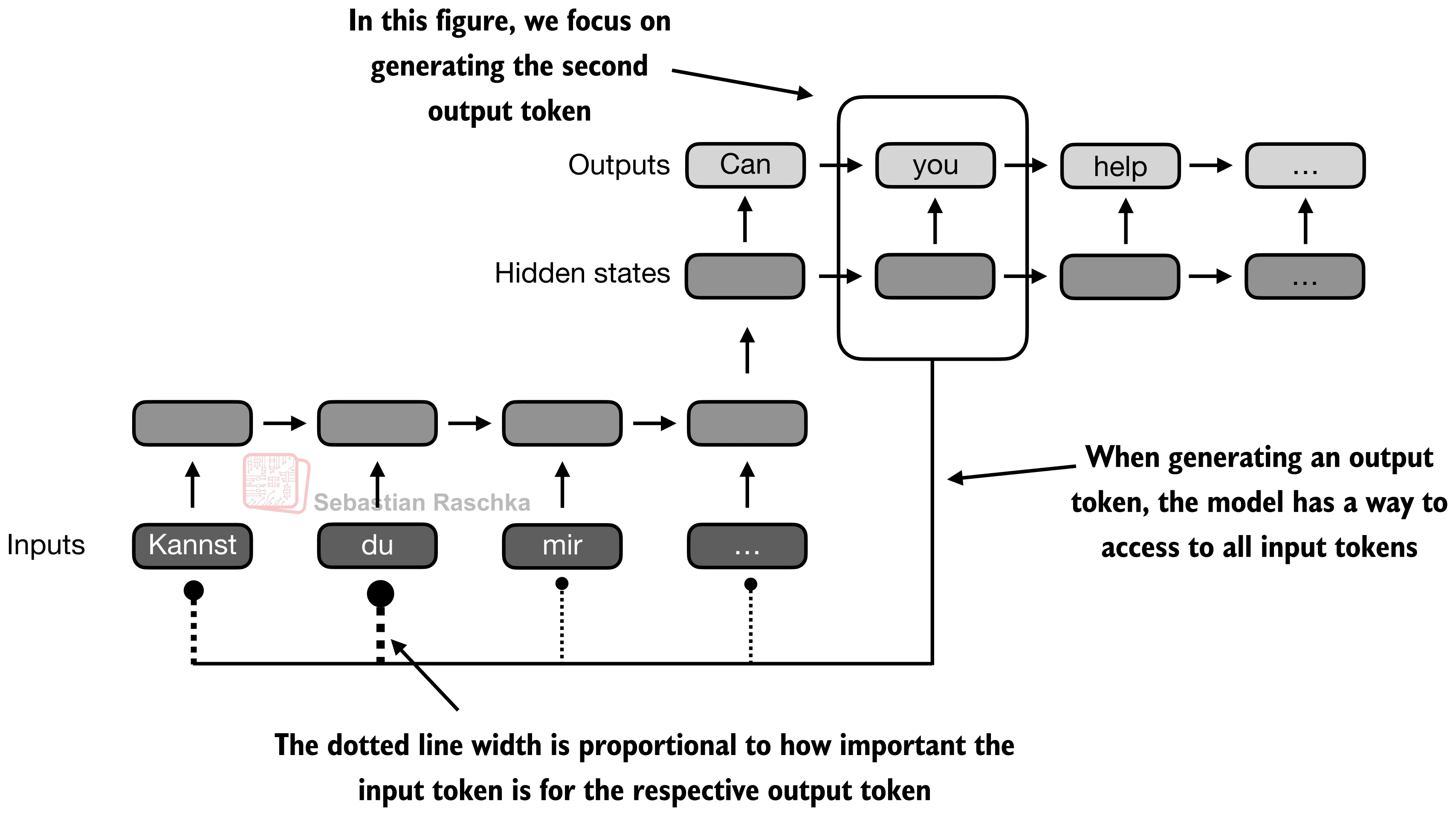
Attention predates transformers and MHA. Its immediate background is encoder-decoder RNNs for translation.
In those older systems, an encoder RNN would read the source sentence token by token and compress it into a sequence of hidden states, or in the simplest version into one final state. Then the decoder RNN had to generate the target sentence from that limited summary. This worked for short and simple cases, but it created an obvious bottleneck once the relevant information for the next output word lived somewhere else in the input sentence.
In short, the limitation is that the hidden state can’t store infinitely much information or context, and sometimes it would be useful to just refer back to the full input sequence.
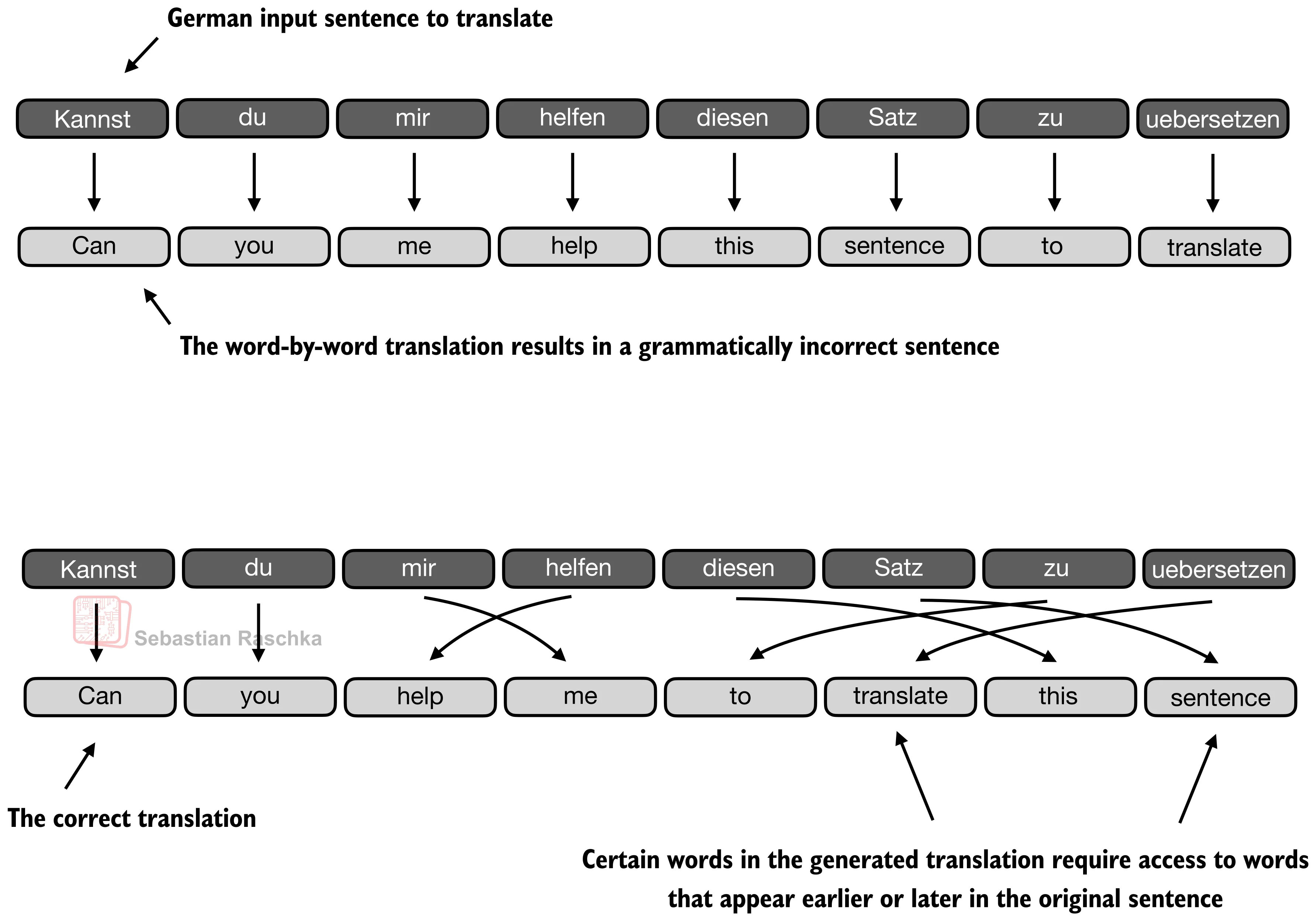
The translation example below shows one of the limitations of this idea. For instance, a sentence can preserve many locally reasonable word choices and still fail as a translation when the model treats the problem too much like a word-by-word mapping. (The top panel shows an exaggerated example where we translate the sentence word by word; obviously, the grammar in the resulting sentence is wrong.) In reality, the correct next word depends on sentence-level structure and on which earlier source words matter at that step. Of course, this could still be translated fine with an RNN, but it would struggle with longer sequences or knowledge retrieval tasks because the hidden state can only store so much information as mentioned earlier.
Figure 4: Translation can fail even when many individual word choices look reasonable because sentence-level structure still matters (Original source LLMs-from-scratch).
The next figure shows that change more directly. When the decoder is producing an output token, it should not be limited to one compressed memory path. It should be able to reach back to the more relevant input tokens directly.
Figure 5: Attention breaks the RNN bottleneck by letting the current output position revisit the full input sequence instead of relying on one compressed state alone (Original source LLMs-from-scratch).
Transformers keep that core idea from the aforementioned attention-modified RNN but remove the recurrence. In the classic Attention Is All You Need paper, attention becomes the main sequence-processing mechanism itself (instead of being just part of an RNN encoder-decoder.)
In transformers, that mechanism is called self-attention, where each token in the sequence computes weights over all other tokens and uses them to mix information from those tokens into a new representation. Multi-head attention is the same mechanism run several times in parallel.
1.3 The Masked Attention Matrix
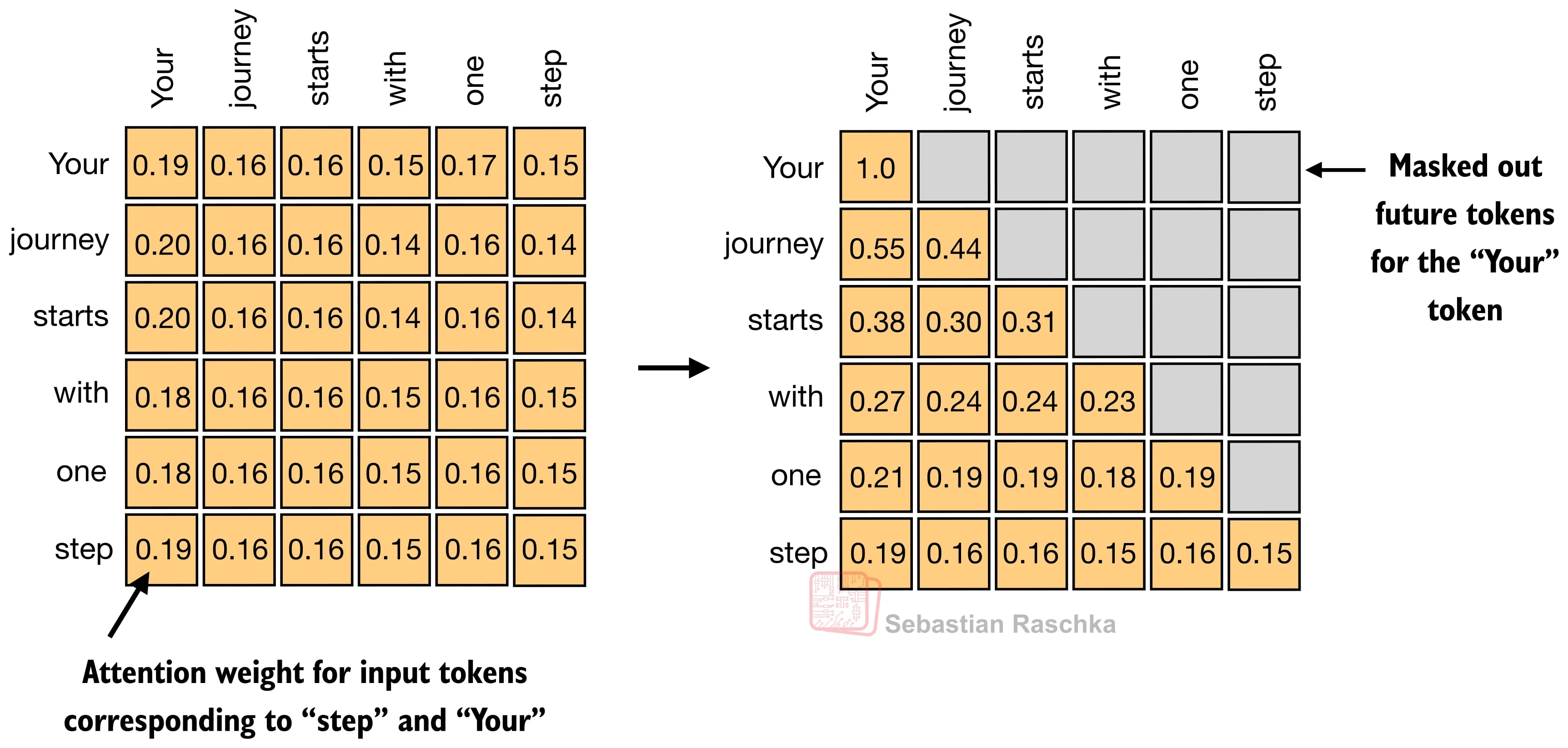
For a sequence of T tokens, attention needs one row of weights per token, so overall we get a T x T matrix.
Each row answers a simple question. When updating this token, how much should each visible token matter? In a decoder-only LLM, future positions are masked out, which is why the upper-right part of the matrix is grayed out in the figure below.
Self-attention is fundamentally about learning these token-to-token weight patterns, under a causal mask, and then using them to build context-aware token representations.
Figure 6: A concrete masked attention matrix where each row belongs to one token, each entry is an attention weight, and future-token entries are removed by the causal mask (Original source Understanding and Coding Self-Attention).
1.4 Self-Attention Internals
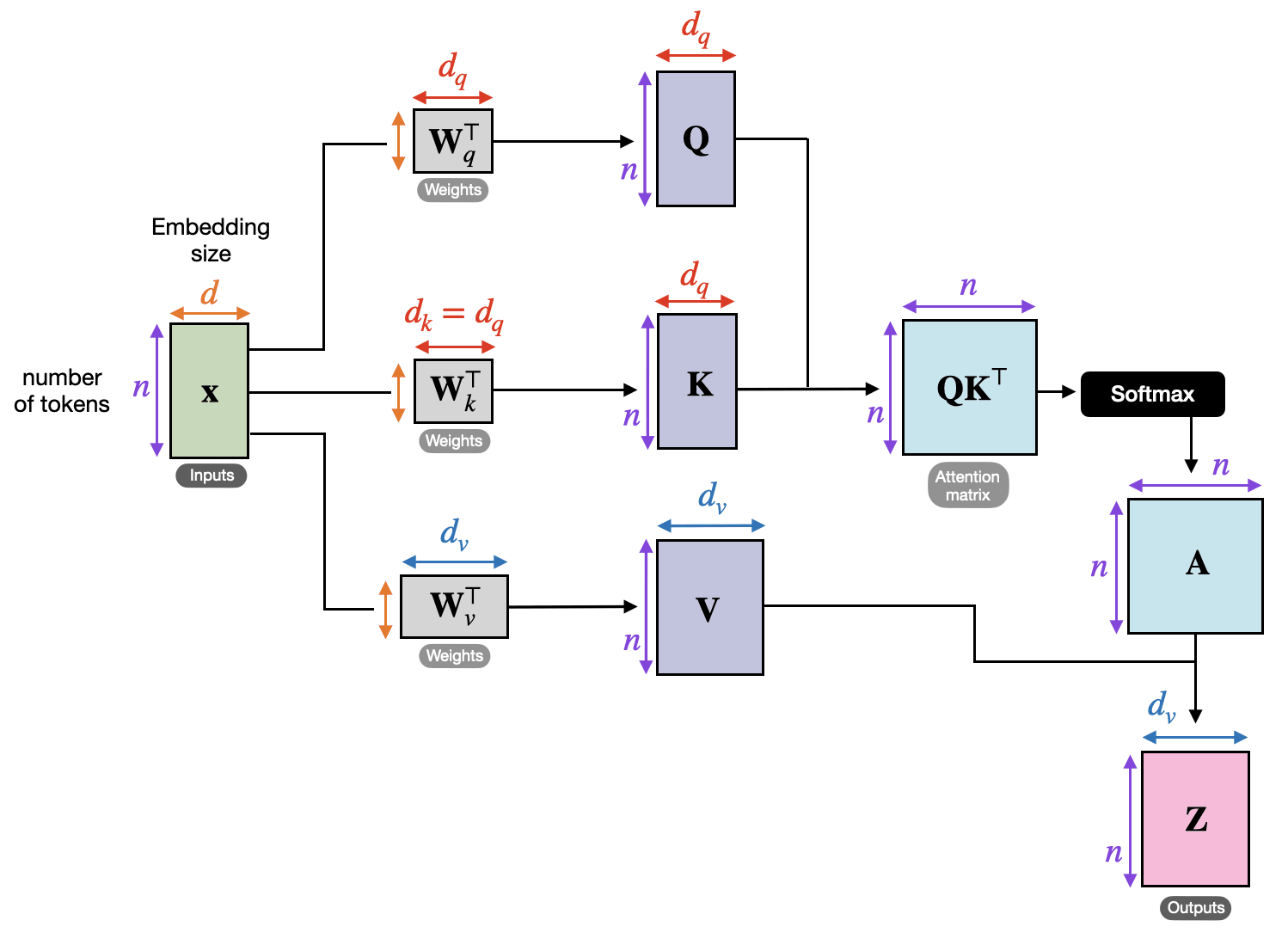
The next figure shows how the transformer computes the attention matrix (A) from the input embeddings X, which is then used to produce the transformed inputs (Z).
Here Q, K, and V stand for queries, keys, and values. The query for a token represents what that token is looking for, the key represents what each token makes available for matching, and the value represents the information that gets mixed into the output once the attention weights have been computed.
The steps are as follows:
Wq, Wk, and Wv are weight matrices that project the input embeddings into Q, K, and V
QK^T produces the raw token-to-token relevance scores
softmax converts those scores into the normalized attention matrix A that we discussed in the previous section
A is applied to V to produce the output matrix Z
Note that the attention matrix is not a separate hand-written object. It emerges from Q, K, and softmax.
Figure 7: The full single-head pipeline, from input embeddings X to the normalized attention matrix A and output representations Z (Original source Understanding and Coding Self-Attention).
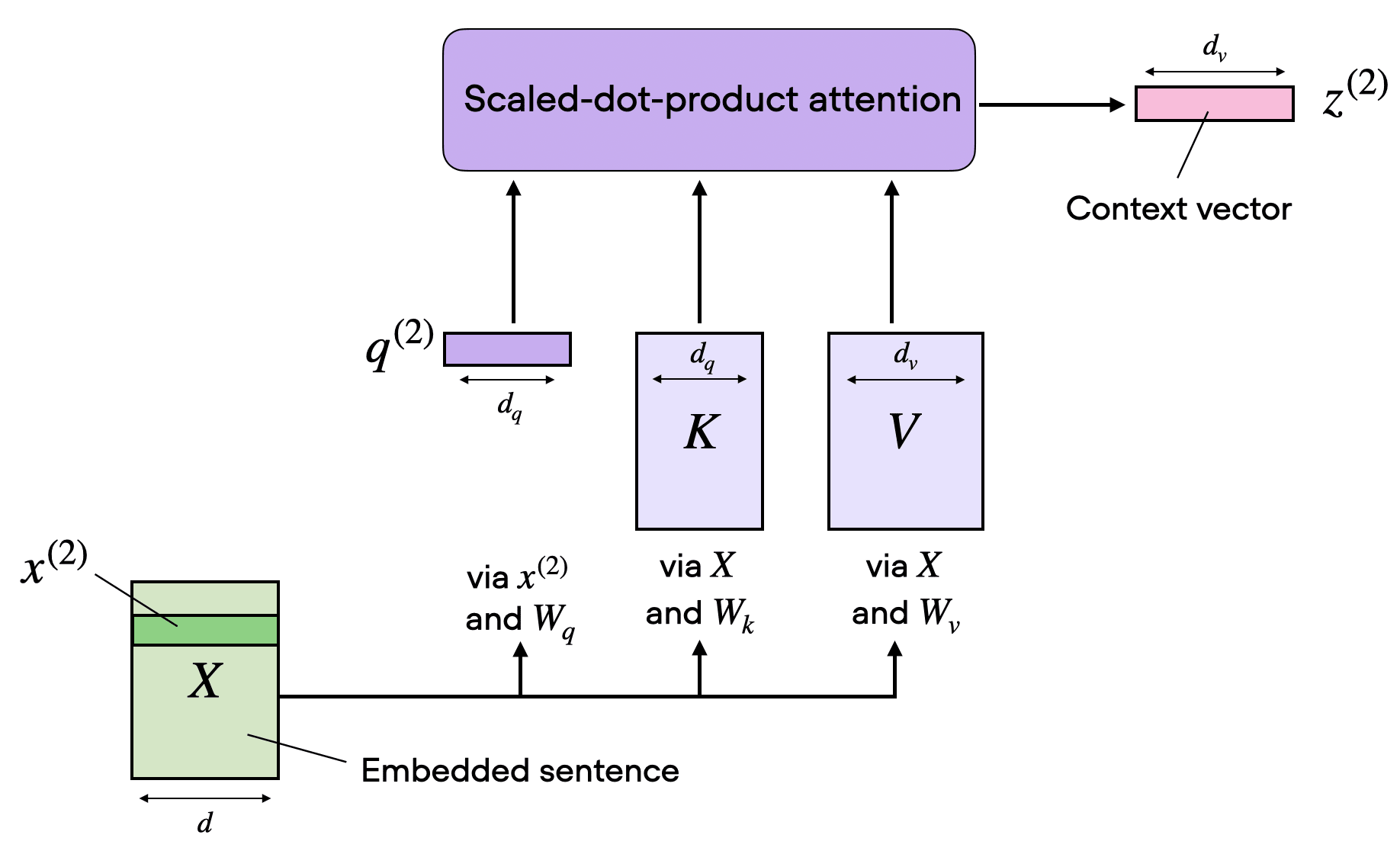
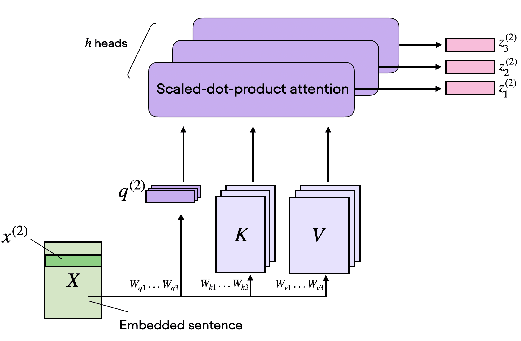
The next figure shows the same concept as the previous figure but the attention matrix computation is hidden inside the “scaled-dot-product attention” box, and we perform the computation only for one input token instead of all input tokens. This is to show a compact form of self-attention with a single head before extending this to multi-head attention in the next section.
Figure 8: One attention head is already a complete mechanism. One set of learned projections produces one attention matrix and one context-aware output stream (Original source Understanding and Coding Self-Attention).
1.5 From One Head To Multi-Head Attention
One set of Wq/Wk/Wv matrices gives us one attention head, which means one attention matrix and one output matrix Z. (This concept was illustrated in the previous section.)
Multi-head attention simply runs several of these heads in parallel with different learned projection matrices.
This is useful because different heads can specialize in different token relationships. One head might focus on short local dependencies, another on broader semantic links, and another on positional or syntactic structure.
Figure 9: Multi-head attention keeps the same basic attention recipe, but repeats it across several heads in parallel so the model can learn several token-to-token patterns at once (Original source Understanding and Coding Self-Attention).
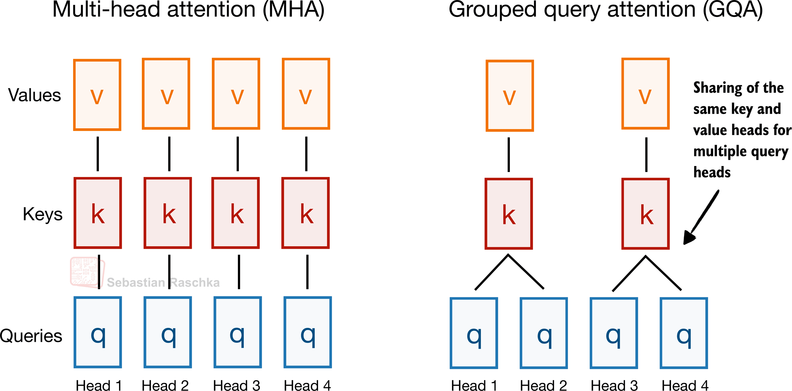
Instead of giving every query head its own keys and values, it lets several query heads share the same key-value projections, which makes KV caching much cheaper (primarily as a memory reduction) without changing the overall decoder recipe very much.
Figure 10: GQA keeps the same overall attention pattern as MHA, but collapses the number of key-value heads by sharing them across multiple query heads (Original source: The Big LLM Architecture Comparison).
In my architecture comparison article, I framed GQA as the new standard replacement for classic multi-head attention (MHA). The reason is that standard MHA gives every head its own keys and values, which is more optimal from a modeling perspective but expensive once we have to keep all of that state in the KV cache during inference.
In GQA, we keep a larger set of query heads, but we reduce the number of key-value heads and let multiple queries share them. That lowers both parameter count and KV-cache traffic without making drastic implementation changes like multi-head latent attention (MLA), which will be discussed later.
In practice, that made and keeps it a very popular choice for labs that wanted something cheaper than MHA but simpler to implement than newer compression-heavy alternatives like MLA.
2.2 GQA Memory Savings
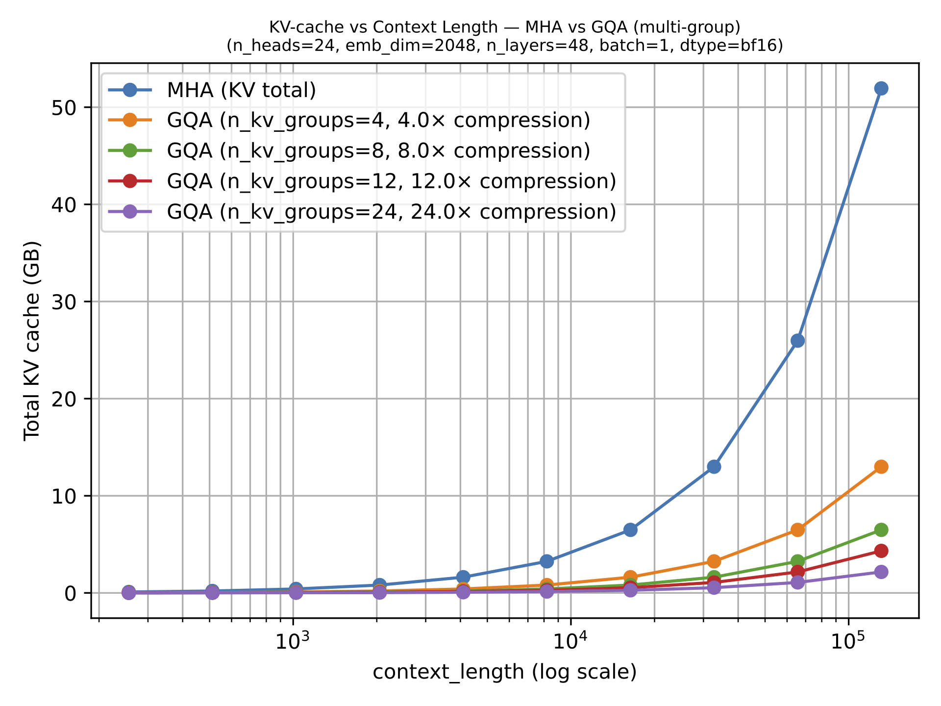
GQA results in big savings in KV storage, since the fewer key-value heads we keep per layer, the less cached state we need per token. That is why GQA becomes more useful as sequence length grows.
GQA is also a spectrum. If we reduce all the way down to one shared K/V group, we are effectively in multi-query attention territory, which is even cheaper but can hurt modeling quality more noticeably. The sweet spot is usually somewhere in between multi-query attention (1 shared group) and MHA (where K/V groups are equal to the number of queries), where the cache savings are large but the modeling degradation relative to MHA stays modest.
More advanced variants such as MLA are becoming popular because they can offer better modeling performance at the same KV efficiency levels (e.g., as discussed in the ablation studies of the DeepSeek-V2 paper), but they also involve a more complicated implementation and a more complicated attention stack.
GQA remains appealing because it is robust, easier to implement, and also easier to train (since there are fewer hyperparameter tunings necessary, based on my experience).
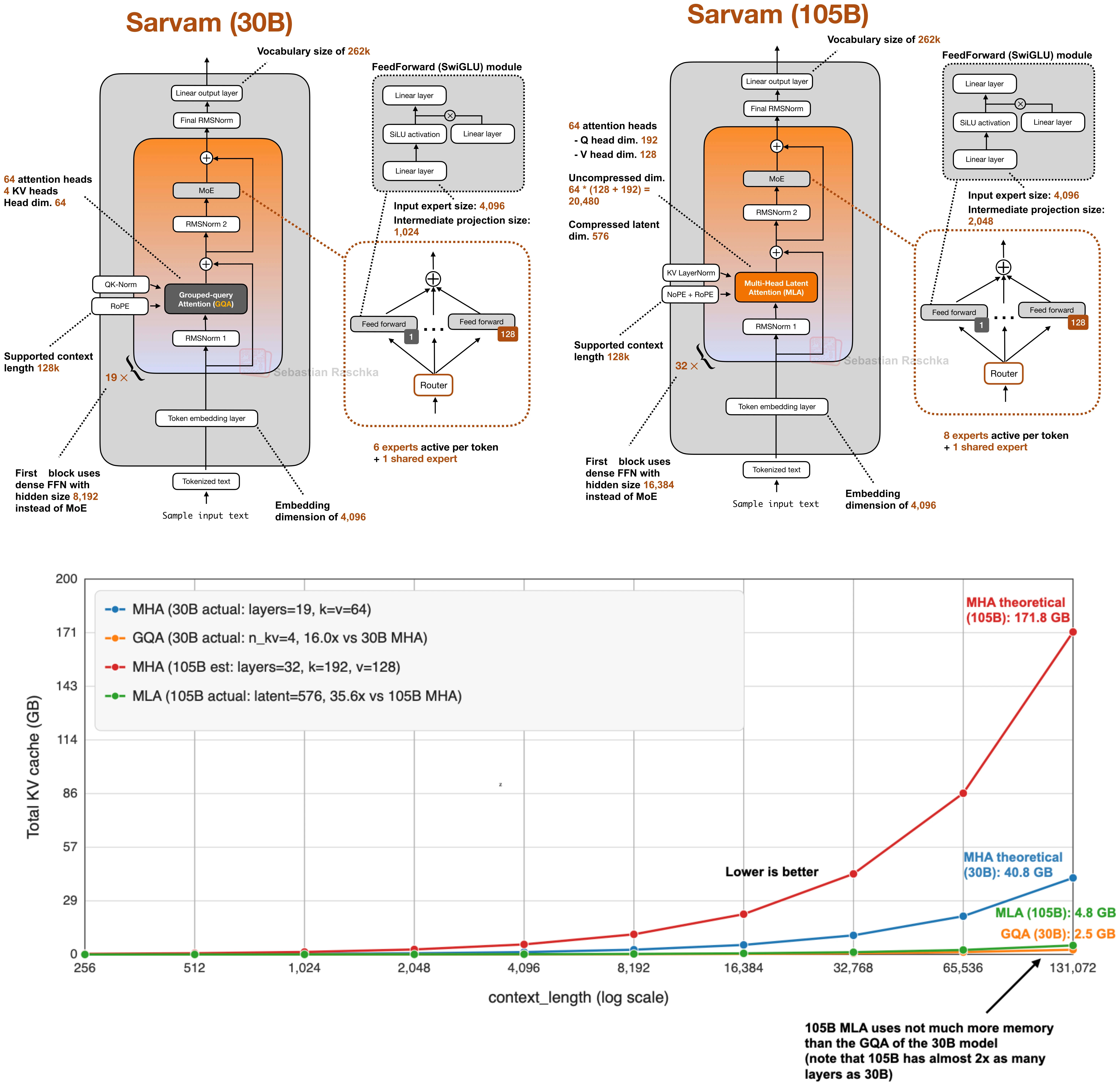
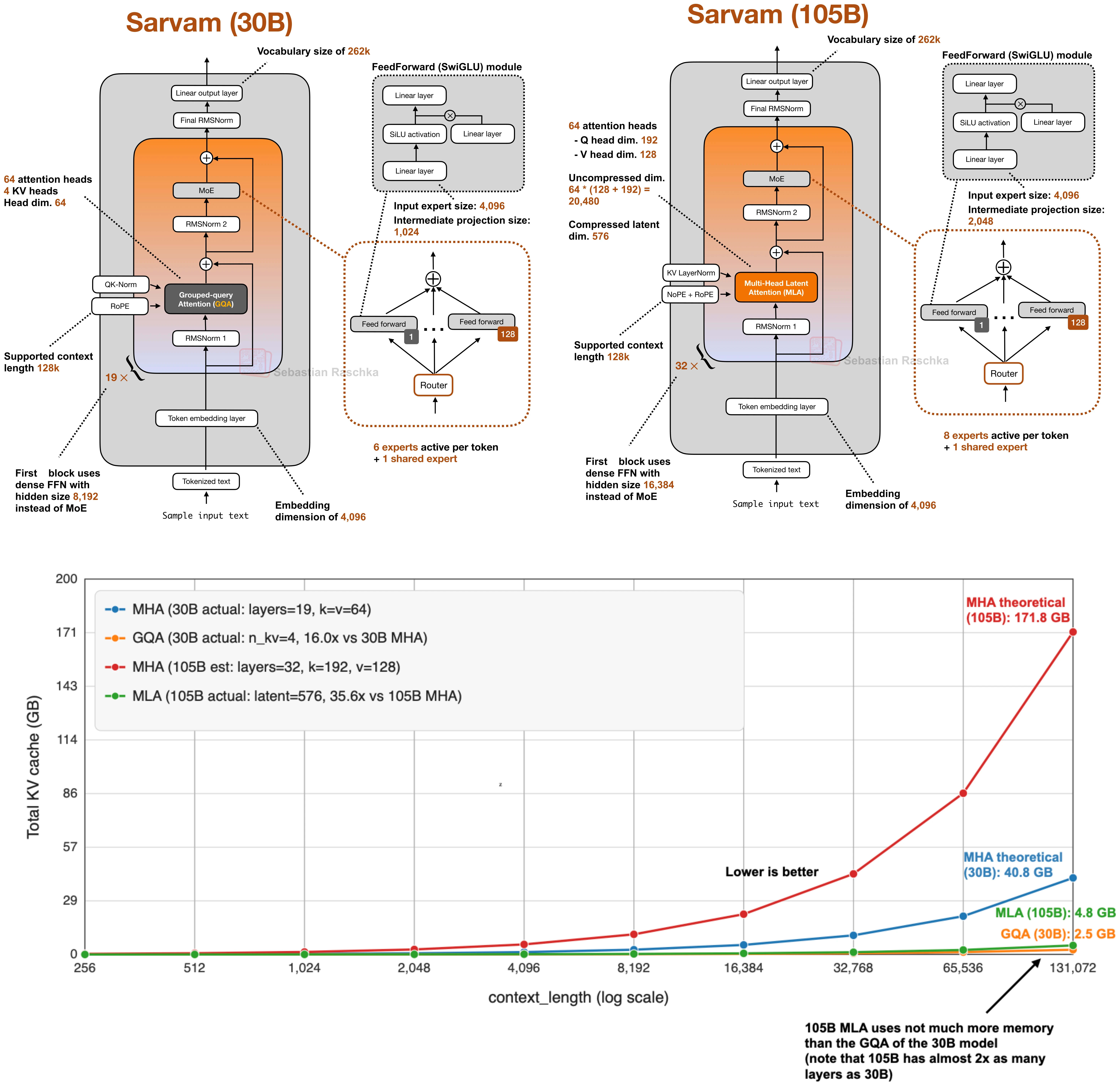
That is why some of the newer releases still stay deliberately classic here. E.g., in my Spring Architectures article, I mentioned that MiniMax M2.5 and Nanbeige 4.1 as models that remained very classic, using only grouped-query attention without piling on other efficiency tricks. Sarvam is a particularly useful comparison point as well: the 30B model keeps classic GQA, while the 105B version switches to MLA.
Figure 12: Total KV cache sizes for 105B Sarvam (using MLA) versus 30B Sarvam (using GQA), versus using plain MHA.
3. Multi-Head Latent Attention (MLA)
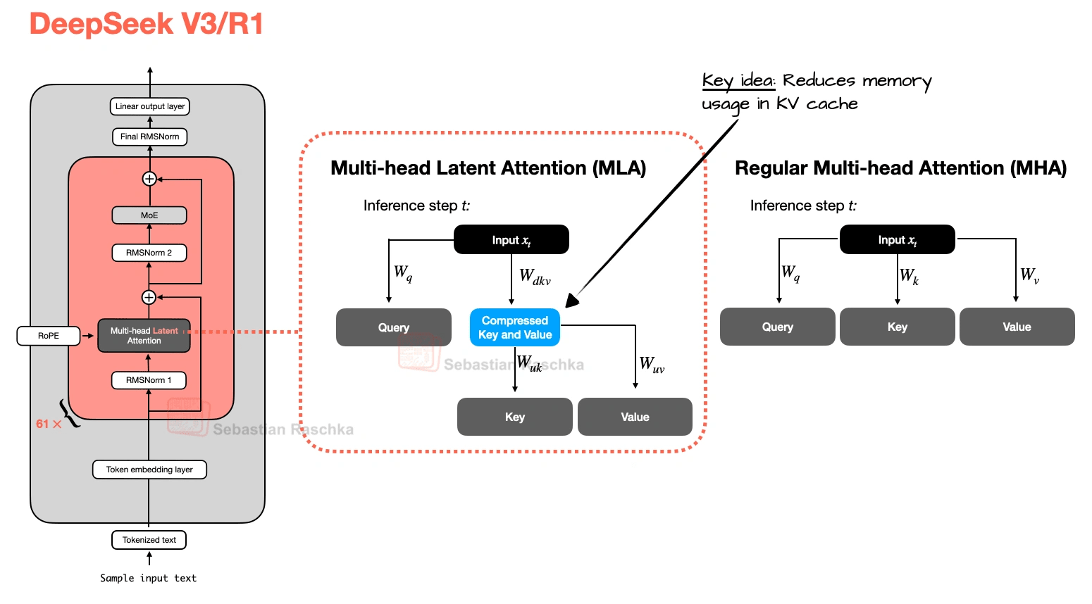
The motivation behind Multi-head Latent Attention (MLA) is similar to Grouped-Query Attention (GQA). Both are solutions for reducing KV-cache memory requirements. The difference between GQA and MLA is that MLA shrinks the cache by compressing what gets stored rather than by reducing how many K/Vs are stored by sharing heads.
Figure 13: Unlike GQA, MLA does not reduce KV cost by grouping heads. It reduces it by caching a compressed latent representation. Note that it is also applied to the query, which is not shown for simplicity (Original source:The Big LLM Architecture Comparison).
MLA, originally proposed in the DeepSeek-V2 paper, became such a defining DeepSeek-era idea (especially after DeepSeek-V3 and R1). It is more complicated to implement than GQA, more complicated to serve, but nowadays also often more compelling once model size and context length get large enough that cache traffic starts to dominate, because at the same rate of memory reduction, it could maintain better modeling performance (more on that later).
Instead of caching full-resolution key and value tensors as in MHA and GQA, MLA stores a latent representation and reconstructs the usable state when needed. Essentially, it is a cache compression strategy embedded inside attention, as illustrated in the previous figure.
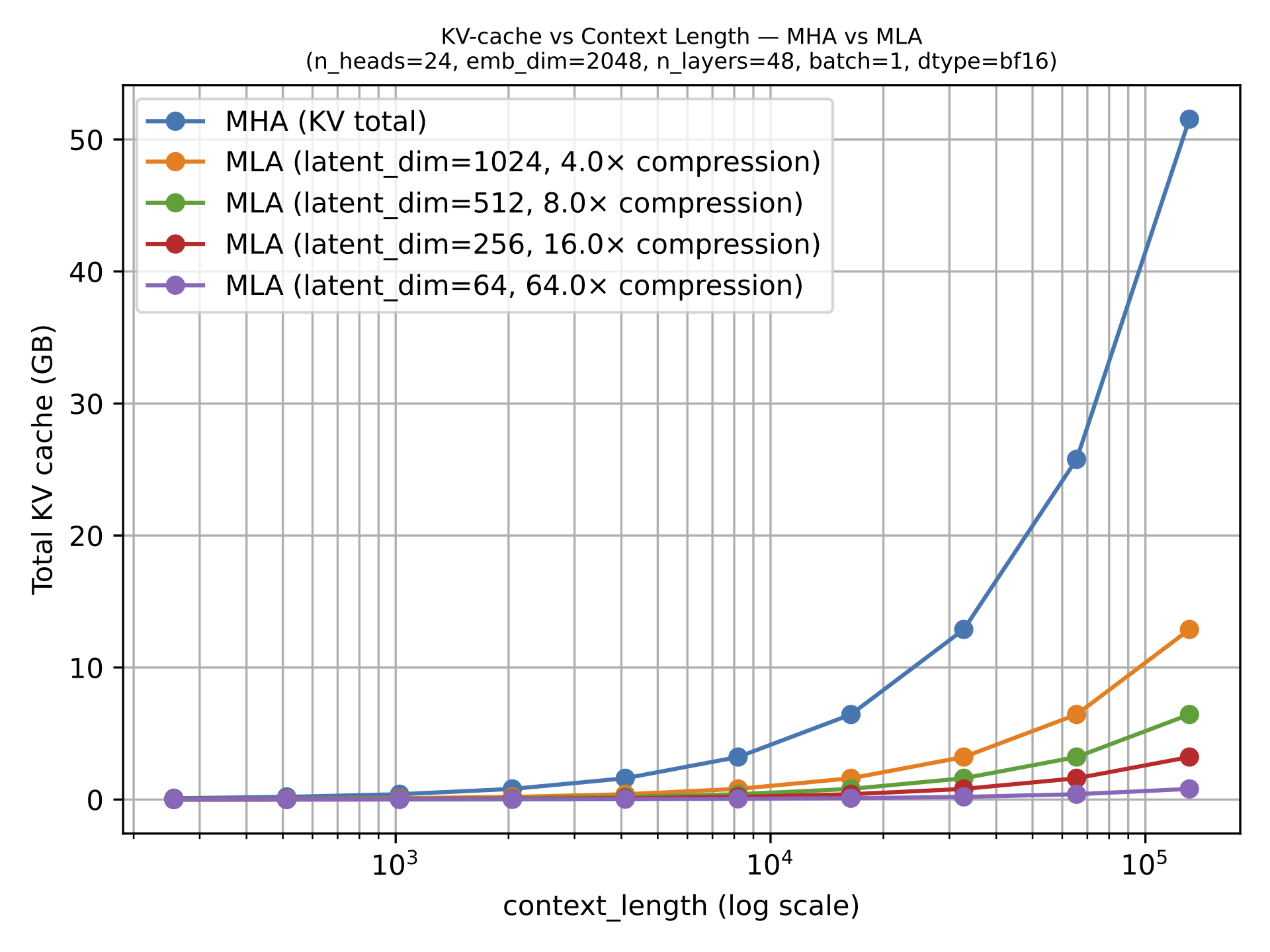
The figure below shows the savings compared to regular MHA.
Figure 14: Once context length grows, the savings from caching a latent representation instead of full K/V tensors become very visible (Original source: LLMs-from-scratch MLA section).
3.2 MLA Ablation Studies
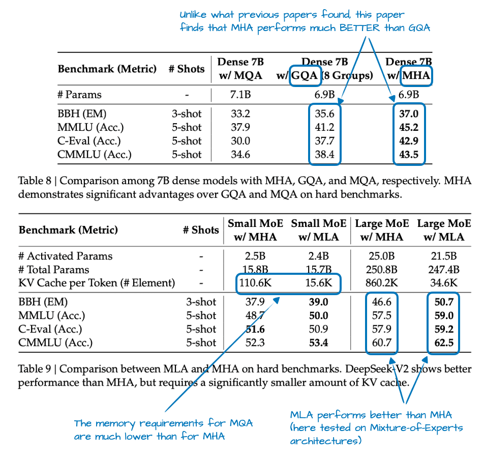
The DeepSeek-V2 paper provided some ablations where GQA looked worse than MHA in terms of modeling performance, while MLA held up much better and could even outperform MHA when tuned carefully. That is a much stronger justification than “it (also) saves memory.”
In other words, MLA is a preferable attention mechanism for DeepSeek not just because it was efficient, but because it looked like a quality-preserving efficiency move at large scale. (But colleagues also told me that MLA only works well at a certain size. For smaller models, let’s say <100B, GQA seems to work better, or, is at least easier to tune and get right.)
Figure 15: GQA drops below MHA here, while MLA remains competitive and can even slightly outperform it. Underlying paper: DeepSeek-V2.
Below is again the comparison between GQA in 30B Sarvam versus MLA in 105B Sarvam.
Figure 16: GQA and MLA are solving the same bottleneck from different directions. The tradeoff is simplicity versus better modeling performance for larger models.
3.3 How MLA Spread After DeepSeek
Once DeepSeek V3/R1, V3.1 etc. normalized the design after its introduction in V2, it started showing up in a second wave of architectures. Kimi K2 kept the DeepSeek recipe and scaled it up. GLM-5 adopted MLA together with DeepSeek Sparse Attention (from DeepSeek V3.2). Ling 2.5 paired MLA with a linear-attention hybrid. Sarvam released two models where the 30B model stayed with classic GQA and the 105B model switched to MLA.
That last pair is particularly useful as it puts the technical-complexity discussion aside. I.e., the Sarvam team implemented both variants and deliberately chose to then use GQA for one variant and MLA for the other. So, in a sense, that makes MLA feel less like a theoretical alternative and more like a concrete architectural upgrade path once a family scales up.
4. Sliding Window Attention (SWA)
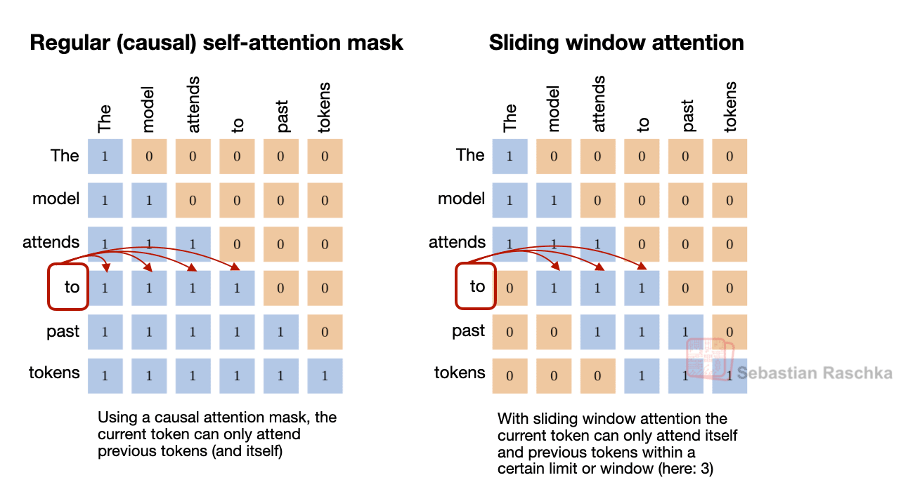
Sliding window attention reduces the memory and compute cost of long-context inference by limiting how many previous tokens each position can attend to. Instead of attending to the entire prefix, each token only attends to a fixed window of recent tokens around its position. Because attention is restricted to a local token neighborhood, this mechanism is often referred to as local attention.
Some architectures combine these local layers with occasional global attention layers so that information can still propagate across the entire sequence.
Figure 17: The conceptual shift is simple. Regular attention is global attention, while sliding-window attention is local attention. Global attention lets every token see the full prefix; SWA turns many of those layers into local attention layers (Original source: The Big LLM Architecture Comparison).
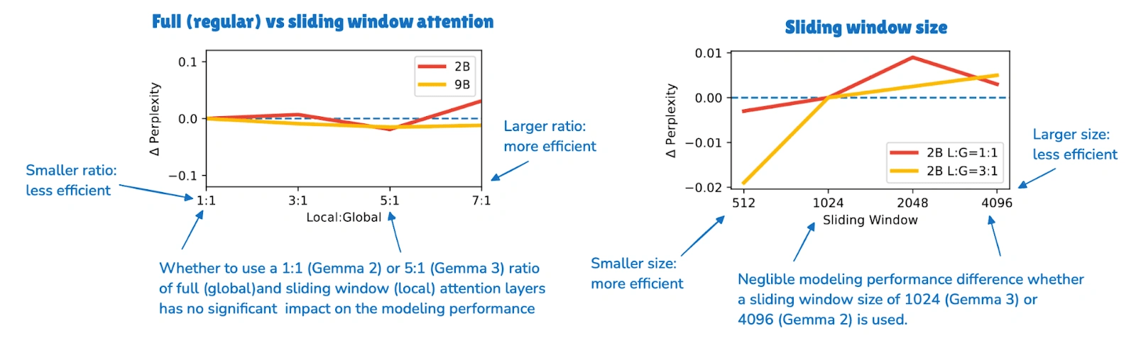
Gemma 3 is still one of the clearest recent SWA examples because it is easy to compare against Gemma 2. Gemma 2 already used a hybrid attention setup with a 1:1 ratio between local and global layers and a 4096-token window. Gemma 3 pushed this further to a 5:1 ratio and reduced the window size to 1024.
The key finding was not that local attention is cheaper, because that was already known. Here, the more interesting takeaway from the Gemma 3 ablation study was that using this more aggressively seemed to hurt modeling performance only slightly.
The Gemma ablation study suggests that the smaller window and more aggressive local:global ratio have little effect on perplexity. Underlying paper: Gemma 3 article (Original source: The Big LLM Architecture Comparison).
4.2 The Ratio And Window Size
In practice, saying that a model “uses SWA” does not mean it relies on SWA alone. What usually matters are the local-to-global layer pattern and the attention window size. For example:
Gemma 3 and Xiaomi use a 5:1 local-to-global pattern.
OLMo 3 and Arcee Trinity use a 3:1 pattern.
Xiaomi also uses a window size of 128, which is much smaller, and therefore more aggressive, than Gemma’s 1024.
SWA is essentially a knob that can be tuned more or less aggressively.
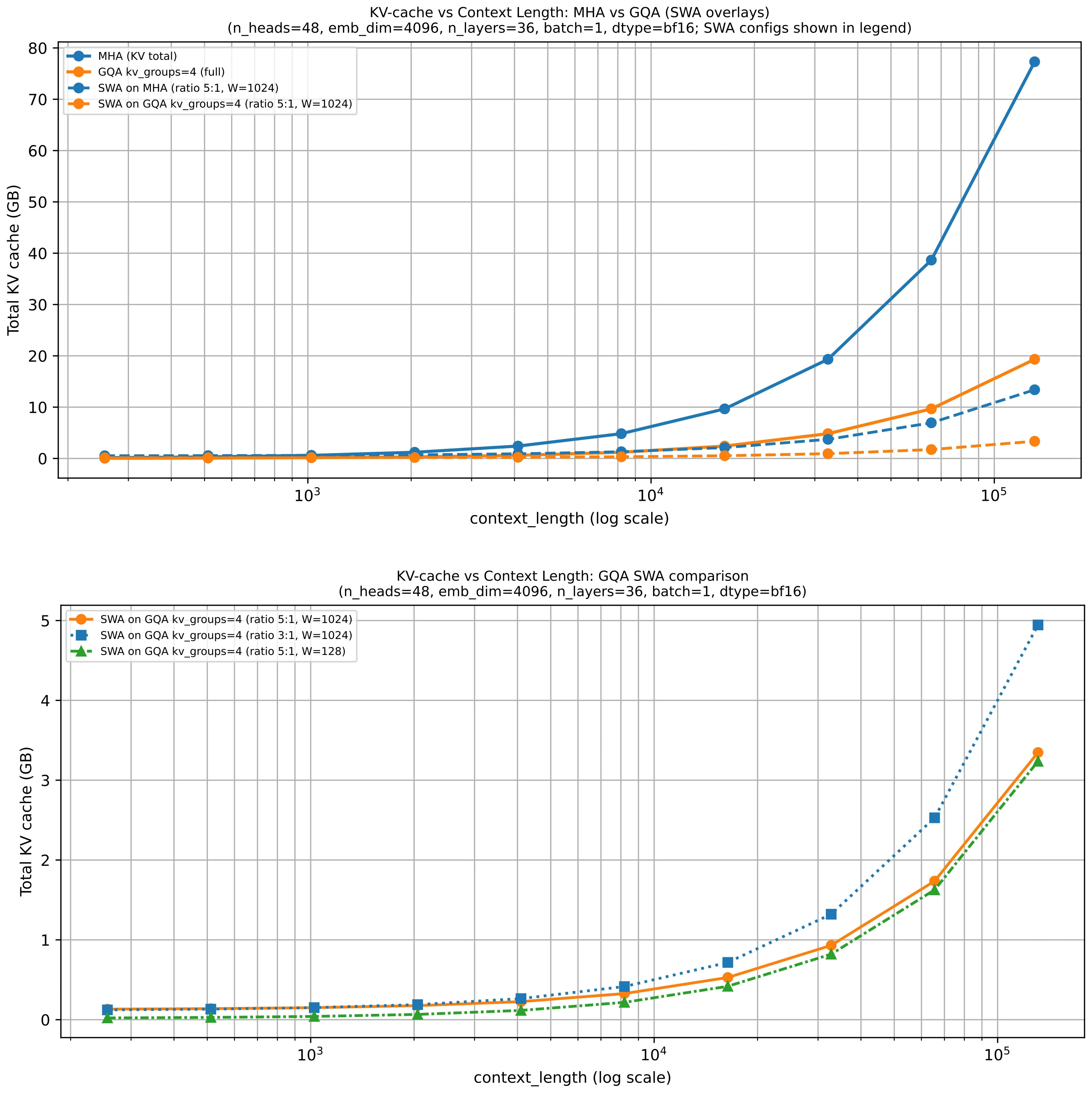
Figure 18: The long-context savings come from turning many full-attention layers into local ones, which reduces how much cached context those layers need to consider (Original source: LLMs-from-scratch SWA materials).
4.3 Combining SWA with GQA
SWA often appears together with GQA because the two ideas address different parts of the same inference problem. SWA reduces how much context a local layer has to consider. GQA reduces how much key-value state each token contributes to the cache.
That is why many recent dense models use both rather than treating them as alternatives. Gemma 3 is again a good reference point here, since it combines sliding window attention with grouped-query attention in the same architecture.
5. DeepSeek Sparse Attention (DSA)
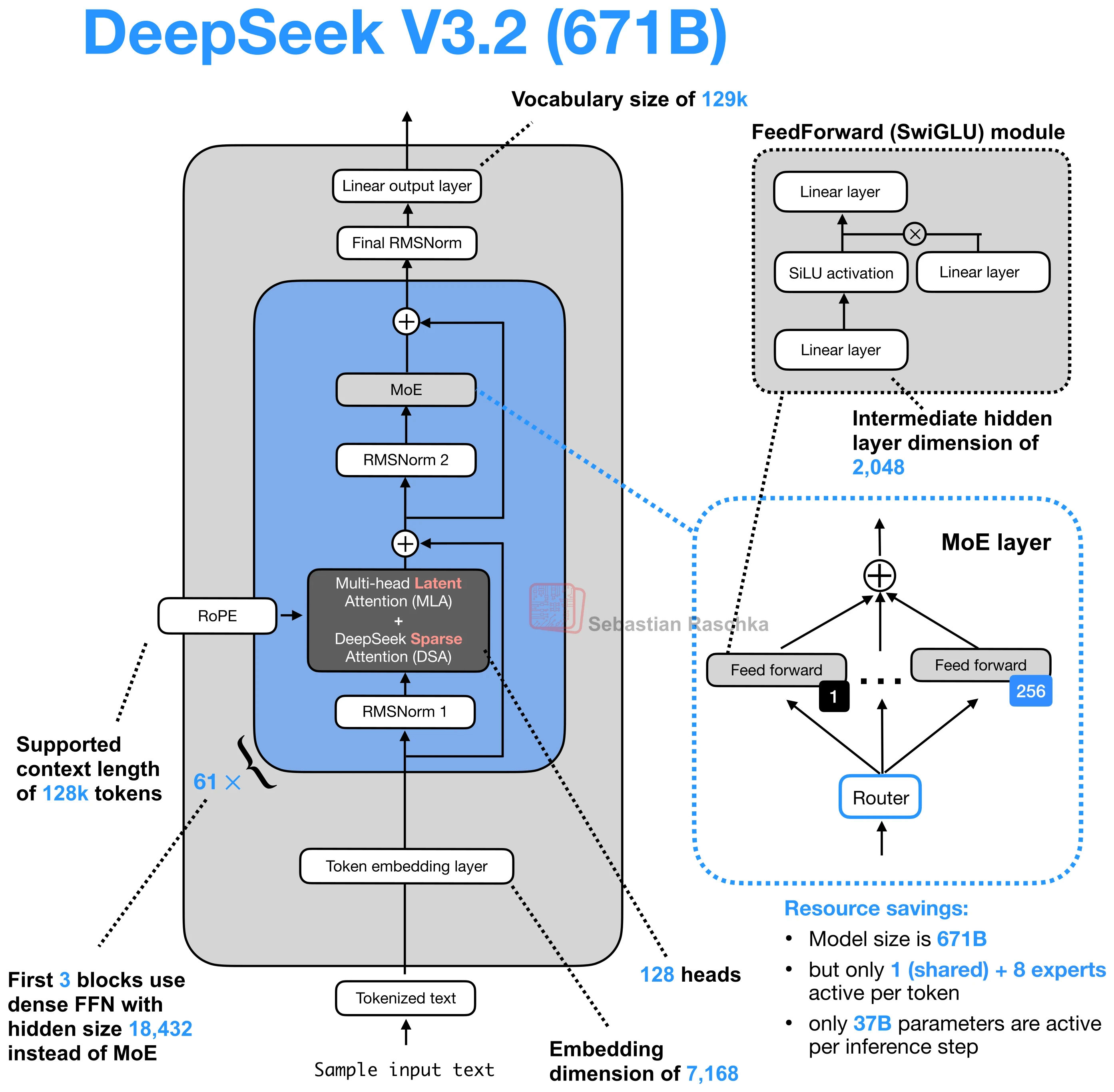
DeepSeek Sparse Attention is one of the architectural changes that appeared in the DeepSeek V3.2 line and later showed up again in GLM-5.
Specifically, DeepSeek V3.2 combines it with Multi-head Latent Attention (MLA), and GLM-5 adopts the same pair for the same general reason, namely, reducing inference cost when context lengths get large.
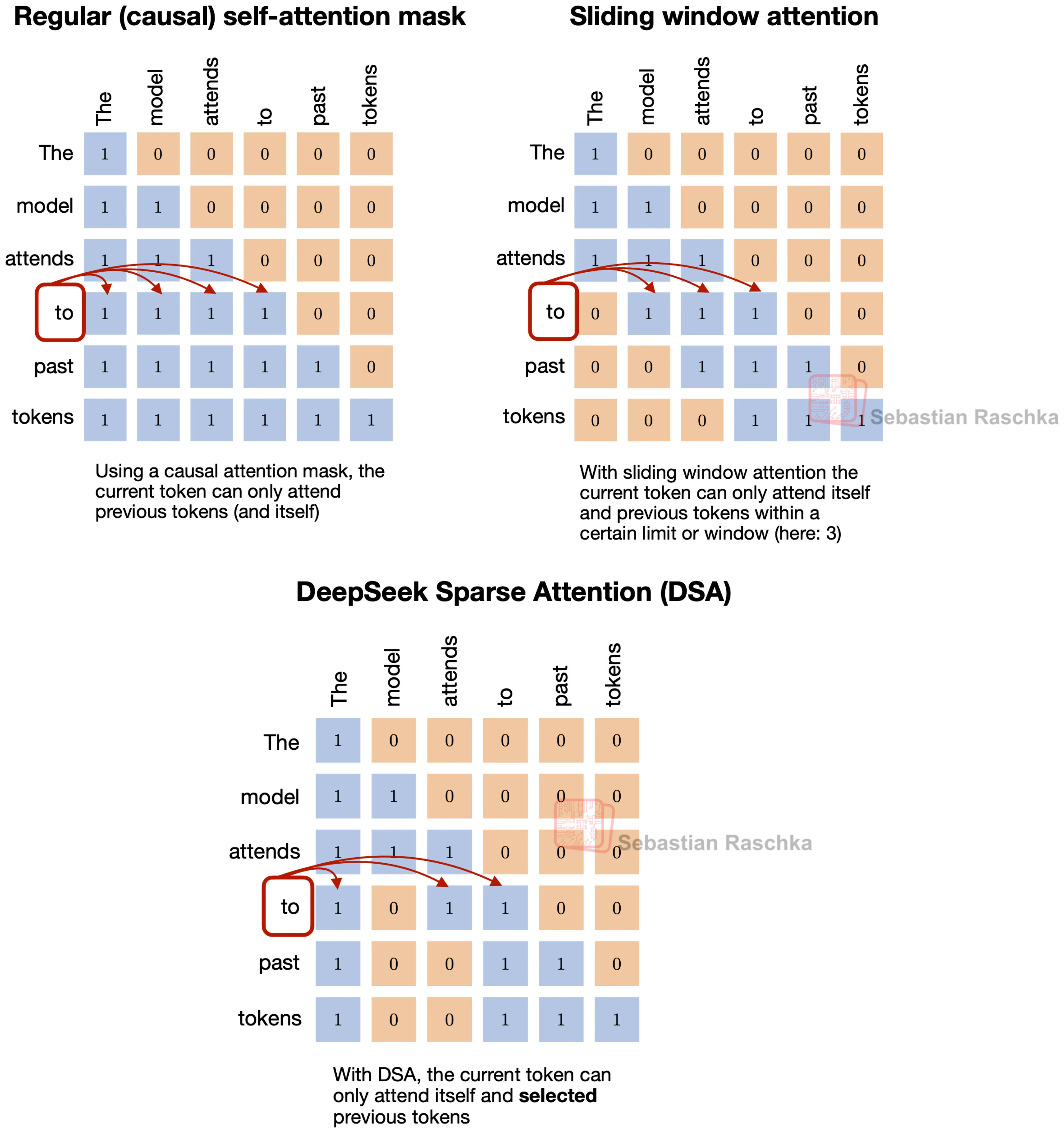
In sliding-window attention, the current token does not attend to the full prefix but only to a fixed local window. This is the same broad idea behind DeepSeek Sparse Attention, where each token also only attends to a subset of previous tokens.
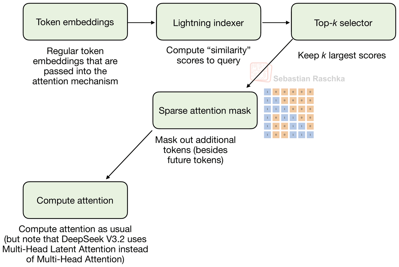
However, the selected tokens are not determined by a fixed-width local window. Instead, DeepSeek Sparse Attention uses a learned sparse pattern. In short, it uses an indexer-plus-selector setup, where a lightning indexer computes relevance scores, and a token selector keeps only a smaller set of high-scoring past positions.
The way the subset of tokens is selected is the main difference from sliding-window attention. Sliding-window attention hard-codes locality. DeepSeek Sparse Attention still limits attention to a subset, but it lets the model decide which prior tokens are worth revisiting.
DeepSeek V3.2 uses both Multi-head Latent Attention (MLA) and DeepSeek Sparse Attention. MLA reduces KV-cache cost by compressing what gets stored. DeepSeek Sparse Attention reduces how much of the prior context the model has to revisit. Put differently, one optimizes the cache representation, the other optimizes the attention pattern on top of it.
Figure 20: DeepSeek V3.2 is the obvious reference point, because this is the model family most closely associated with the sparse-attention idea.
The sparse pattern is not random. The first stage is a lightning indexer that scores previous tokens for each new query token. It uses MLA’s compressed token representations and computes a learned similarity score over the prior context, so the model can rank which earlier positions are worth revisiting.
The second stage is a token selector. It keeps only a smaller high-scoring subset, for example, a top-k set of past positions, and turns that subset into the sparse attention mask. So the main point is that DeepSeek Sparse Attention does not hard-code the sparsity pattern. It learns which past tokens to keep.
DeepSeek Sparse Attention is relatively new and relatively complicated to implement, which is why it has not been so widely adopted as Grouped-Query Attention (GQA) yet.
6. Gated Attention
Gated attention is best understood as a modified full-attention block rather than as a separate attention family.
It usually appears inside hybrid stacks that still keep an occasional full-attention layer for exact content retrieval, but add a few stability-oriented changes on top of an otherwise familiar scaled dot-product attention block.
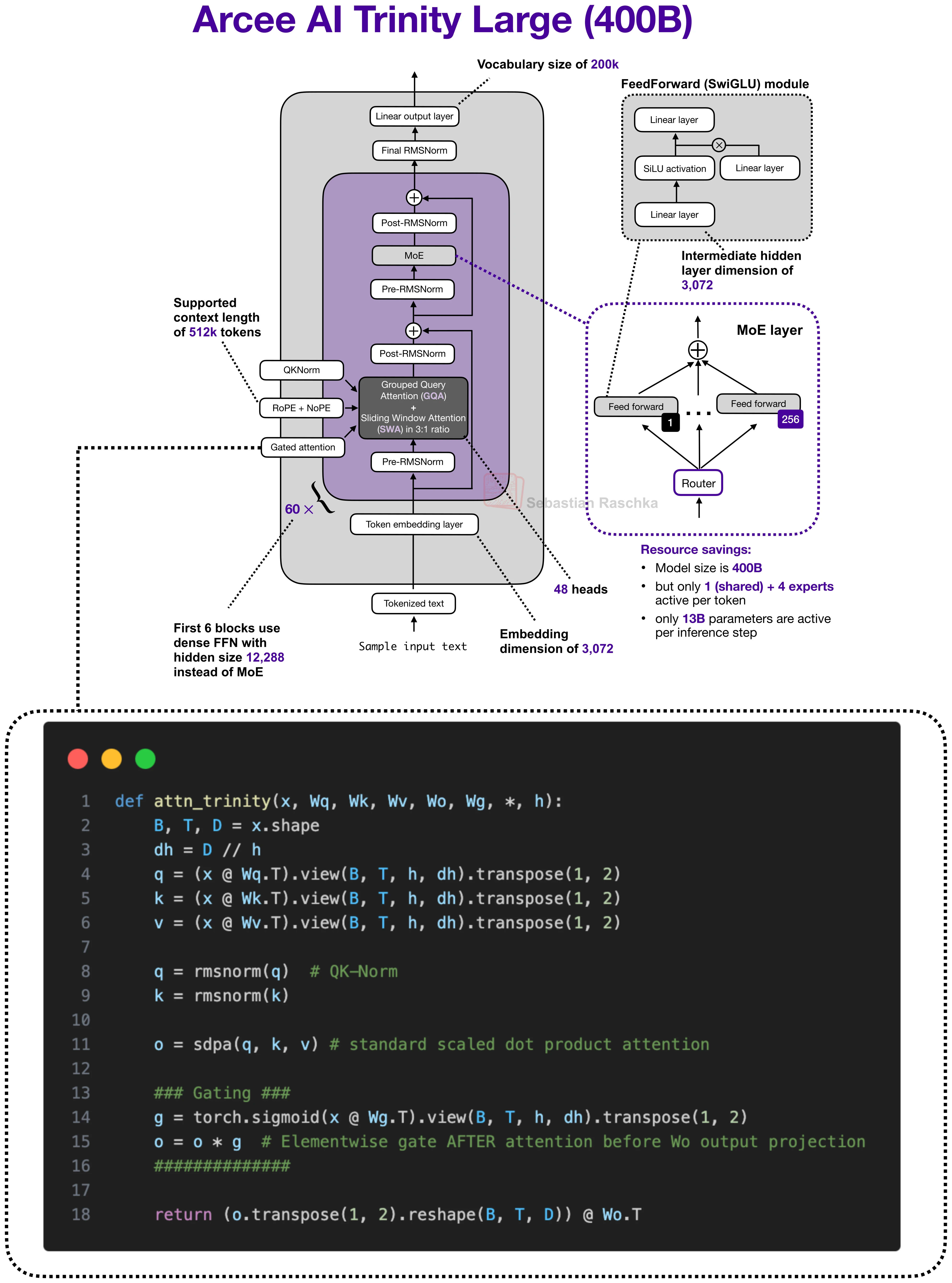
Figure 22: Trinity Large is a useful comparison because gated attention is not only a Qwen idea (more on that later). Here the gate appears after the scaled dot-product attention output and before the output projection in a different long-context architecture (Original source: A Dream of Spring for Open-Weight LLMs).
6.1 Where Gated Attention Appears
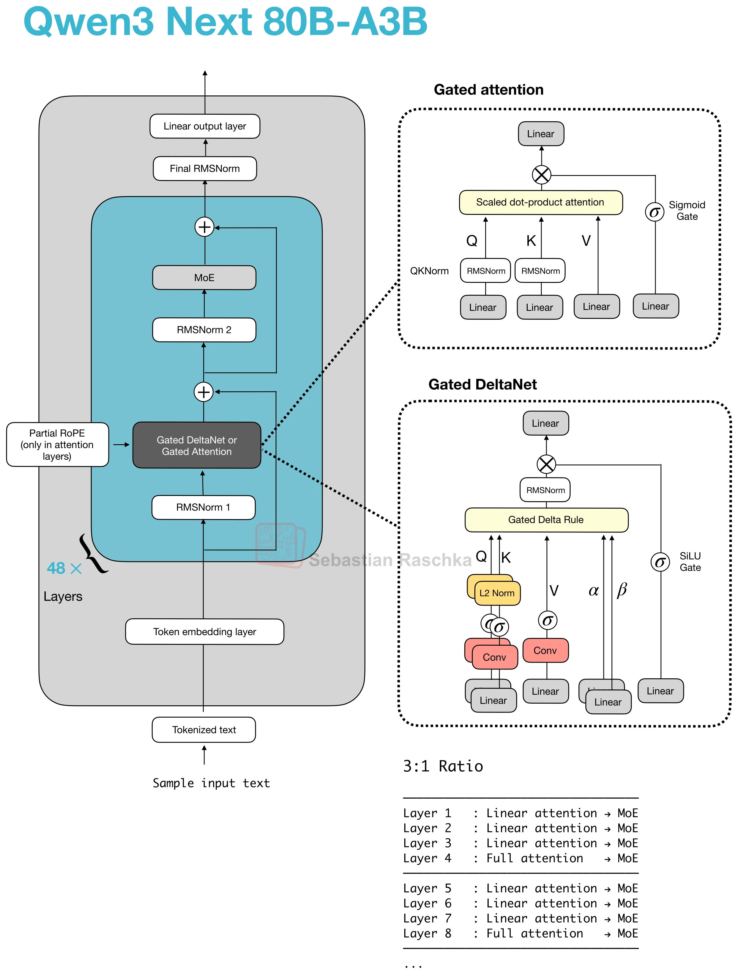
The Qwen3-Next and Qwen3.5 architectures show that recent hybrids (covered in the next section) do not replace attention everywhere. Instead, they replace most attention layers with a cheaper alternative and keep a smaller number of full-attention layers in the stack.
Those remaining full-attention layers are where gated attention typically appears. Qwen3-Next and Qwen3.5 use it together with Gated DeltaNet in a 3:1 pattern.
But hybrid architectures aside, Trinity uses a related gating idea in a more conventional attention stack, as shown in the previous figure above.
6.2 Gated Attention Relative To Standard Attention
The gated attention block in Qwen-style hybrids or Trinity (not a hybrid) is essentially standard scaled-dot-product attention with a few changes on top. In the original Gated Attention paper, those changes are presented as a way to make the retained full-attention layers behave more predictably inside a hybrid stack.
The block still looks like standard (full) attention, but it adds:
an output gate that scales the attention result before it is added back to the residual,
a zero-centered QK-Norm variant instead of standard RMSNorm for q and k,
partial RoPE.
These are not changes on the scale of MLA or linear attention but merely stability and control changes applied to an otherwise familiar attention block.
Figure 23: In Qwen3-Next and Qwen3.5, gated attention appears as the full-attention layer that periodically breaks up runs of Gated DeltaNet blocks.
Note that the figure above also includes Gated DeltaNet, which we will cover in the next section below.
7. Hybrid Attention
Hybrid attention is a broader design pattern rather than a specific, single mechanism. The overall idea is to keep a transformer-like stack, but replace most of the expensive full-attention layers with cheaper linear or state-space sequence modules.
The motivation is long-context efficiency. Full attention grows quadratically with sequence length, so once models move to contexts like 128k, 256k, or 1M tokens, attention memory and compute become expensive enough that using cheaper sequence modules in most layers while keeping only a smaller number of heavier retrieval layers starts making more sense. (Note that this comes with a bit of a modeling performance trade-off, though.)
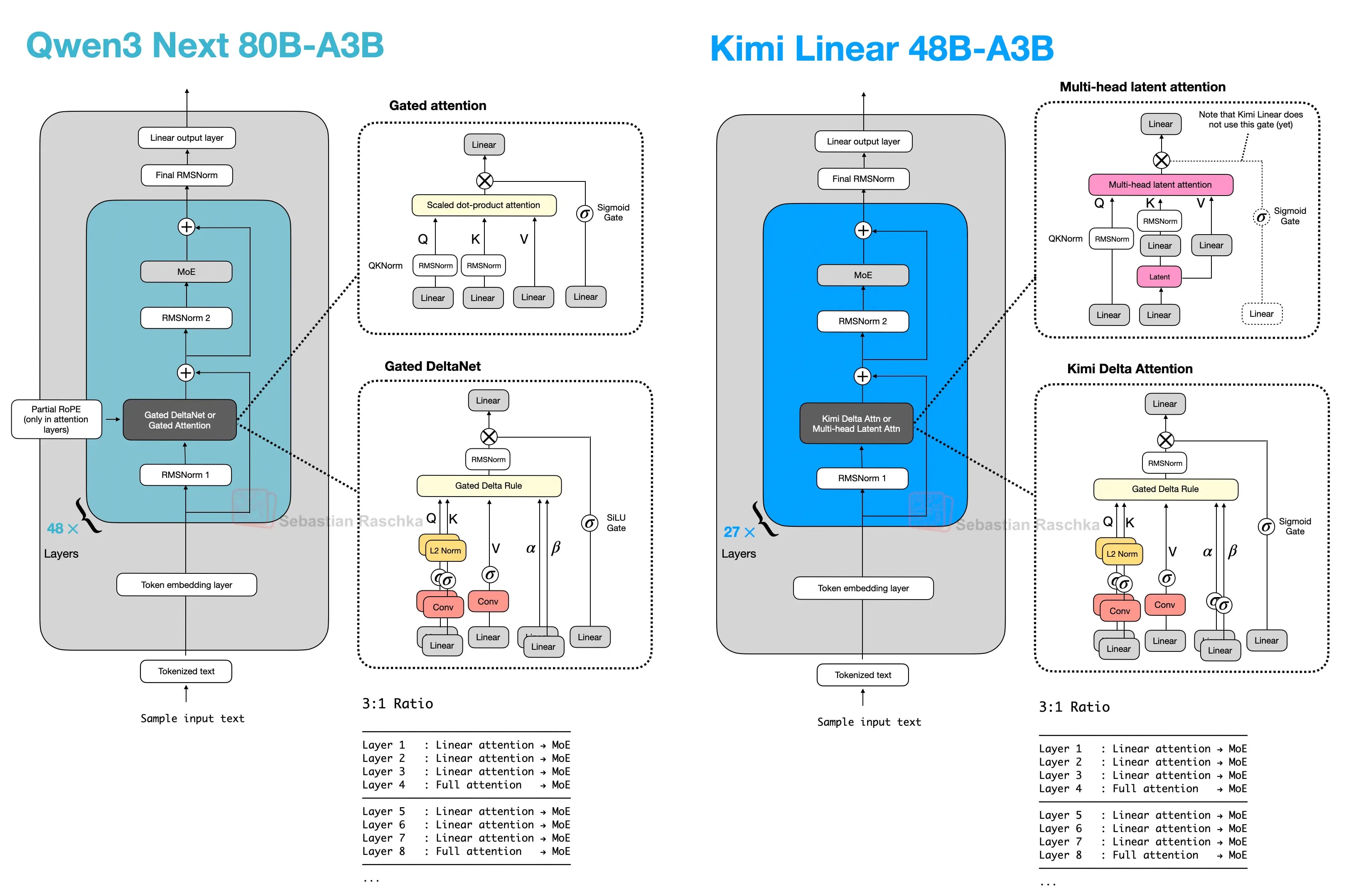
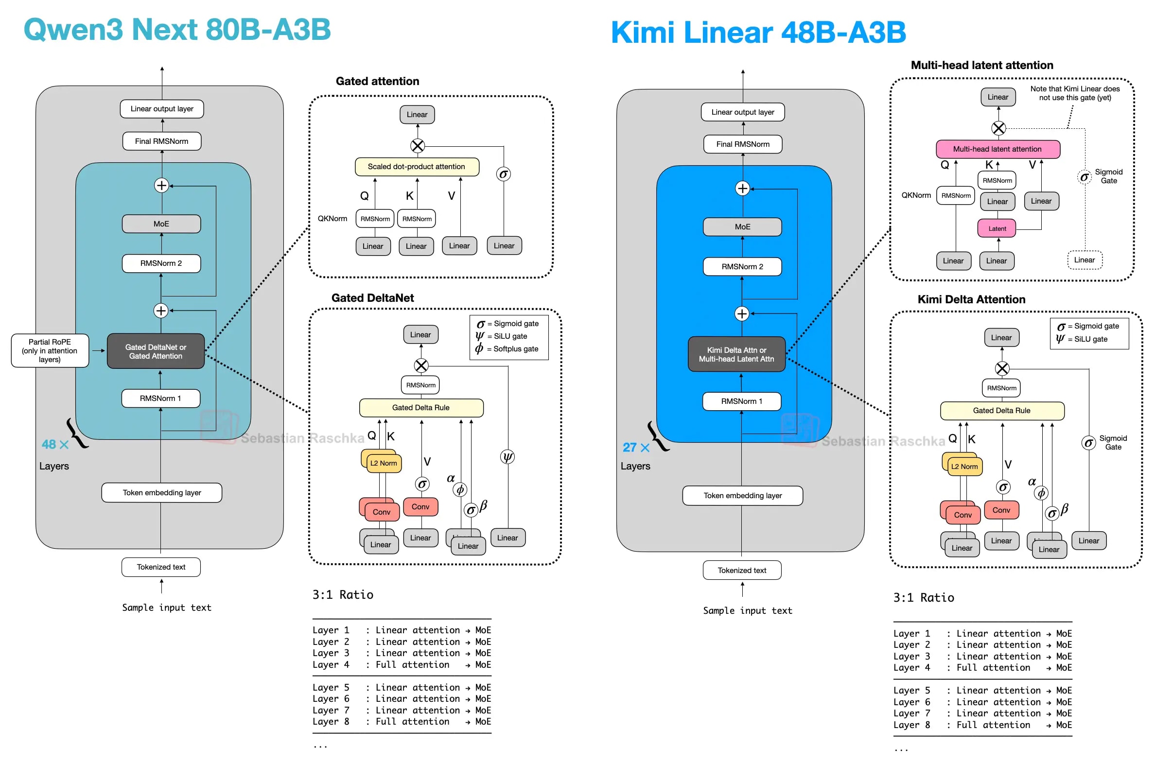
In Qwen3-Next, this pattern appears as a 3:1 mix of Gated DeltaNet and Gated Attention blocks. Gated DeltaNet is also closely related to Mamba-2 (see the Gated Delta Networks: Improving Mamba2 with Delta Rule paper, for instance), and the mechanism can be read as a DeltaNet-style fast-weight update combined with Mamba-style gating. Later architectures keep the same overall idea but swap in other lightweight sequence mixers, such as Kimi Delta Attention, Lightning Attention, or standard Mamba-2.
Figure 24: The basic hybrid pattern, where most blocks are cheaper sequence mixers and every fourth block restores a heavier attention layer (Original source The Big LLM Architecture Comparison).
7.1 Gated DeltaNet in Qwen3-Next
To my knowledge, the first prominent example of a close-to-flagship LLM with hybrid attention was Qwen3-Next in 2025, which does not remove attention completely but mixes three Gated DeltaNet blocks with one Gated Attention block.
Here, lightweight Gated DeltaNet blocks do most of the long-context work and keep memory growth much flatter than full attention. The heavier gated-attention layer remains because DeltaNet is less exact at content-based retrieval.
Inside a Gated DeltaNet block, the model computes query, key, and value vectors together with two learned gates (α, β). Rather than forming the usual token-to-token attention matrix, it writes to a small fast-weight memory using a delta-rule update. In rough terms, the memory stores a compressed running summary of past information, while the gates control how much new information is added and how much previous state is retained.
That makes Gated DeltaNet a linear-attention or recurrent-style mechanism rather than just another tweak to MHA. Relative to Mamba-2, the close connection is that both belong to the linear-time gated sequence-model family, but Gated DeltaNet uses a DeltaNet-style fast-weight memory update instead of the Mamba state-space update.
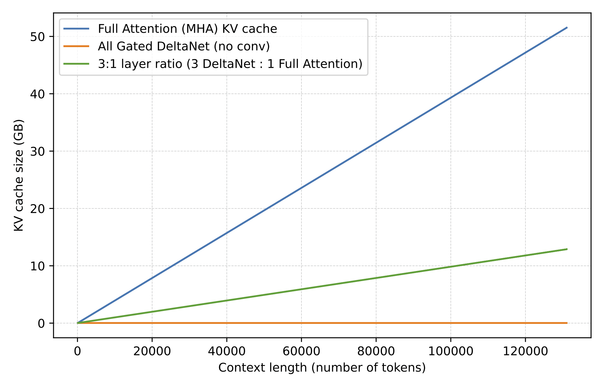
Figure 25: The practical motivation behind the hybrids is shown here in the memory curve. Hybrid stacks with Gated DeltaNet grow much more slowly with context length than ordinary full attention (Original source LLMs-from-scratch DeltaNet materials).
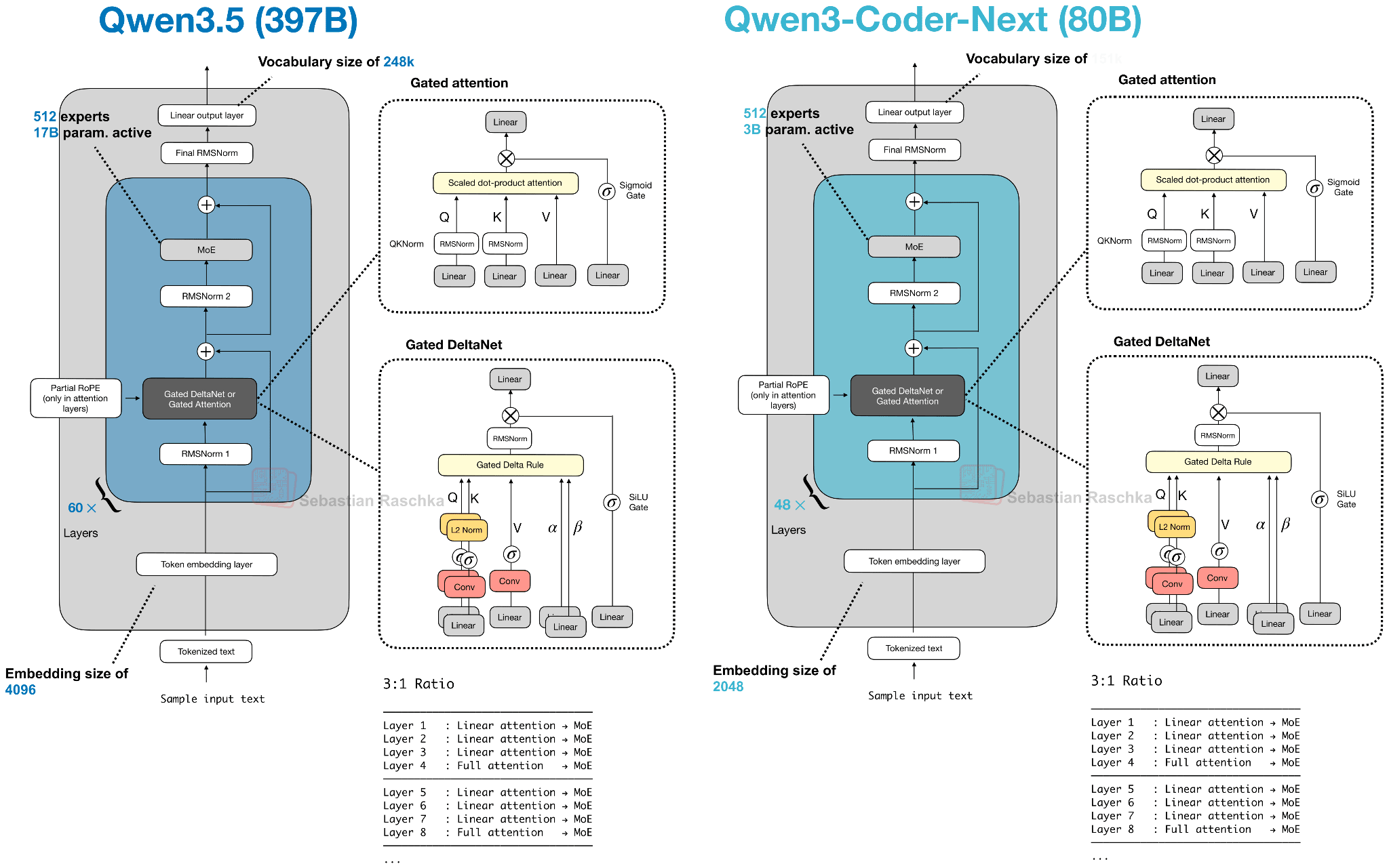
Qwen3.5 moves the former Qwen3-Next hybrid into Qwen’s main flagship series, which is an interesting move. This basically signals that the hybrid strategy is a success and that we may see more models with this architecture in the future.
Figure 26: Qwen3.5 shows the Qwen team promoting the former Qwen3-Next side-branch into the main model line rather than leaving it as a one-off efficiency variant (Original source A Dream of Spring for Open-Weight LLMs).
7.2 Kimi Linear And Modified Delta Attention
Kimi Linear keeps the same broad transformer skeleton and the same 3:1 pattern, but it changes both halves of the recipe.
On the lightweight side, Kimi Delta Attention is a refinement of Gated DeltaNet. Where Qwen3-Next uses a scalar gate per head to control memory decay, Kimi uses channel-wise gating, which gives finer control over the memory update. On the heavier side, Kimi replaces Qwen3-Next’s gated-attention layers with gated MLA layers.
So, it’s still the same broader pattern as in Qwen3-Next and Qwen3.5, but both ingredients (slightly) change. I.e., most layers are still handled by a cheaper linear-style mechanism, and periodic heavier layers still remain for stronger retrieval.
Figure 27: Kimi Linear keeps the same overall hybrid pattern while changing both the lightweight side and the heavier attention side of the stack (Original source The Big LLM Architecture Comparison).
7.3 Ling 2.5 And Lightning Attention
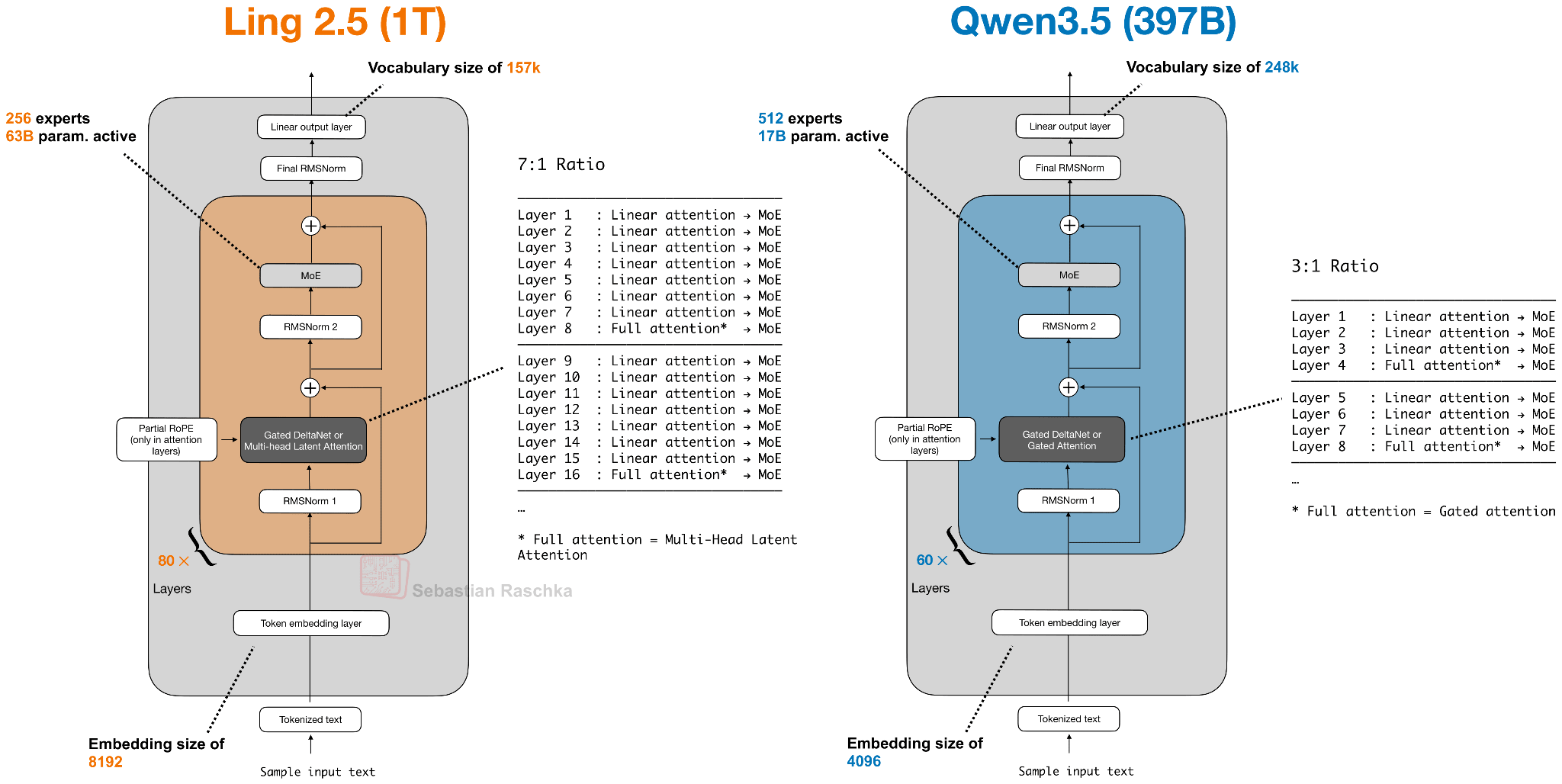
Ling 2.5 shows another swap on the lightweight side. Instead of Gated DeltaNet, Ling uses a slightly simpler recurrent linear attention variant called Lightning Attention. On the heavier side, it keeps MLA from DeepSeek.
Most sequence mixing happens in the cheaper linear-attention blocks, while a smaller number of heavier layers remain to preserve stronger retrieval. The difference is that the specific lightweight mechanism is now Lightning Attention rather than DeltaNet or Kimi Delta Attention.
Figure 28: Ling 2.5 and Qwen3.5 are both linear-attention hybrids, even though Ling swaps in Lightning Attention and MLA instead of the Qwen recipe (Original source A Dream of Spring for Open-Weight LLMs).
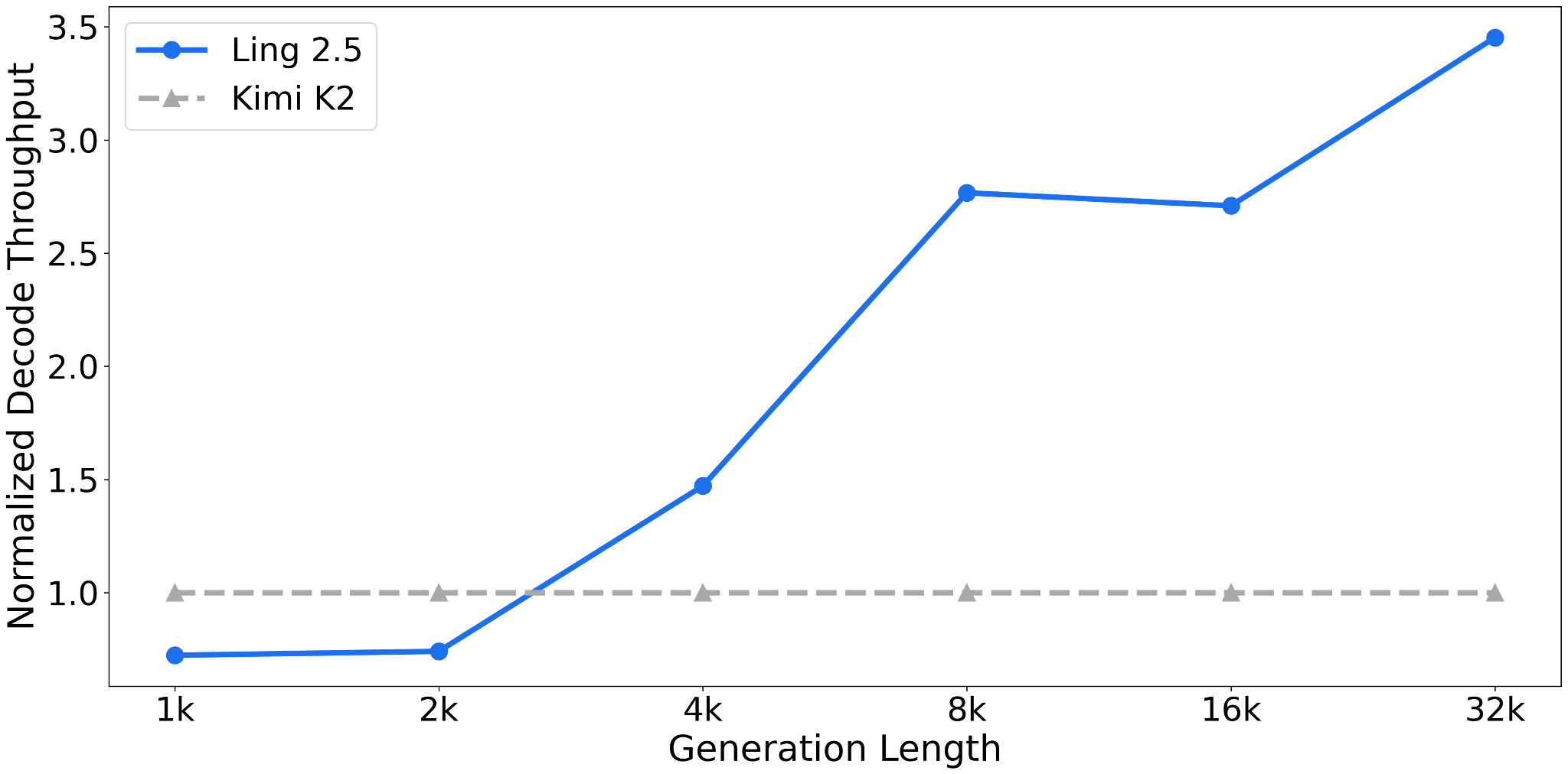
Ling 2.5 is aimed more at long-context efficiency than at absolute benchmark leadership. According to the Ling team, it was reported as substantially faster than Kimi K2 at 32k tokens, which is the practical payoff these hybrids are aiming for.
Figure 29: Ling 2.5 was presented as a strong efficiency upgrade, with much higher 32k-token throughput than Kimi K2 at the same 1-trillion-parameter scale (Original source Ling 2.5 model hub page).
Nemotron And Mamba-2
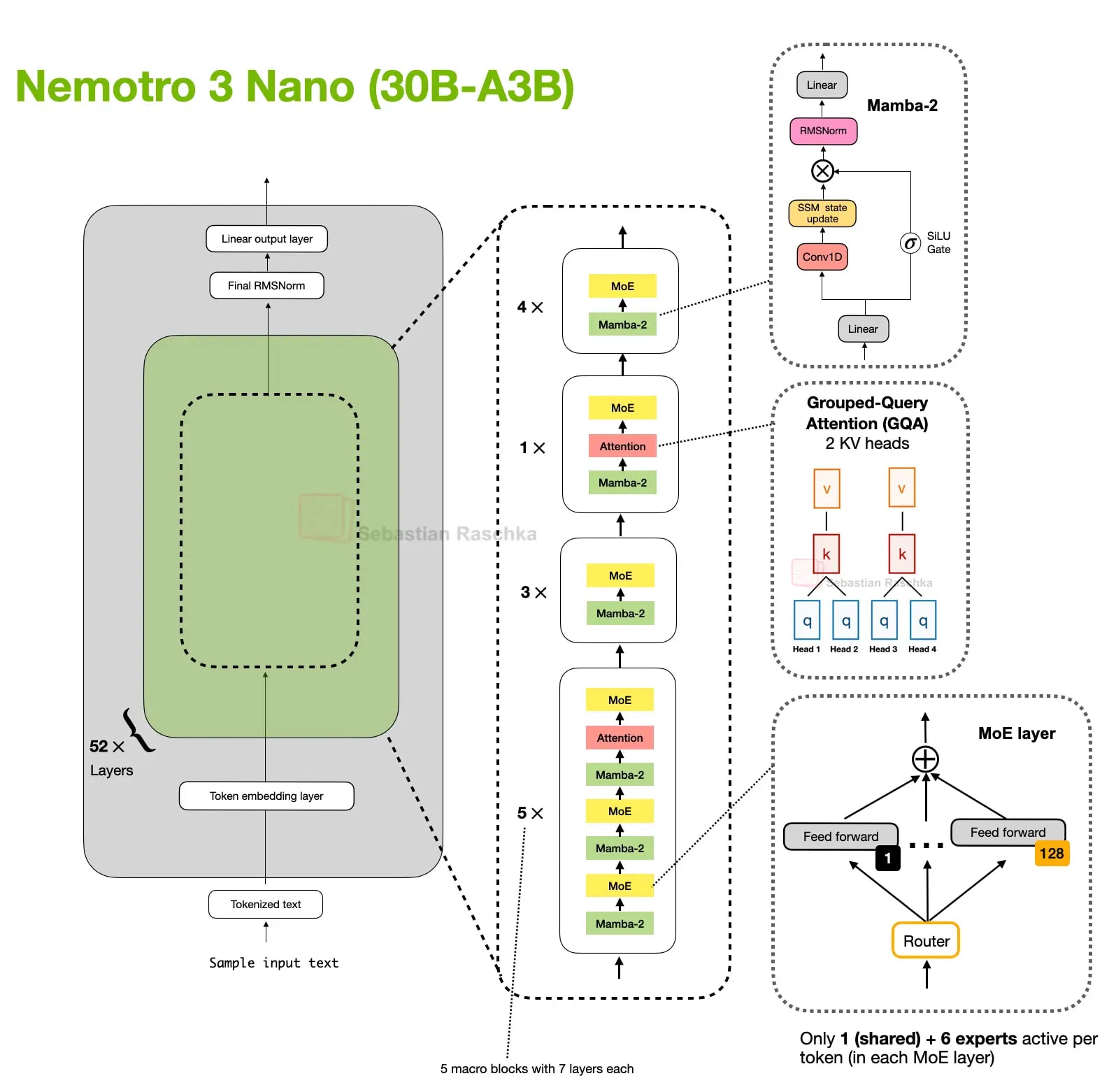
Nemotron pushes the pattern further away from the transformer baseline. Nemotron 3 Nano is a Mamba-Transformer hybrid that interleaves Mamba-2 sequence-modeling blocks with sparse MoE layers and uses self-attention only in a small subset of layers.
This is a more extreme version of the same basic tradeoff discussed above. Here, the lightweight sequence module is a Mamba-2 state-space block rather than a DeltaNet-style fast-weight update, but the basic tradeoff is similar.
Figure 30: Nemotron 3 Nano uses Mamba-2 for most of the sequence modeling work, with self-attention only appearing in a small subset of layers (Original source The Big LLM Architecture Comparison).
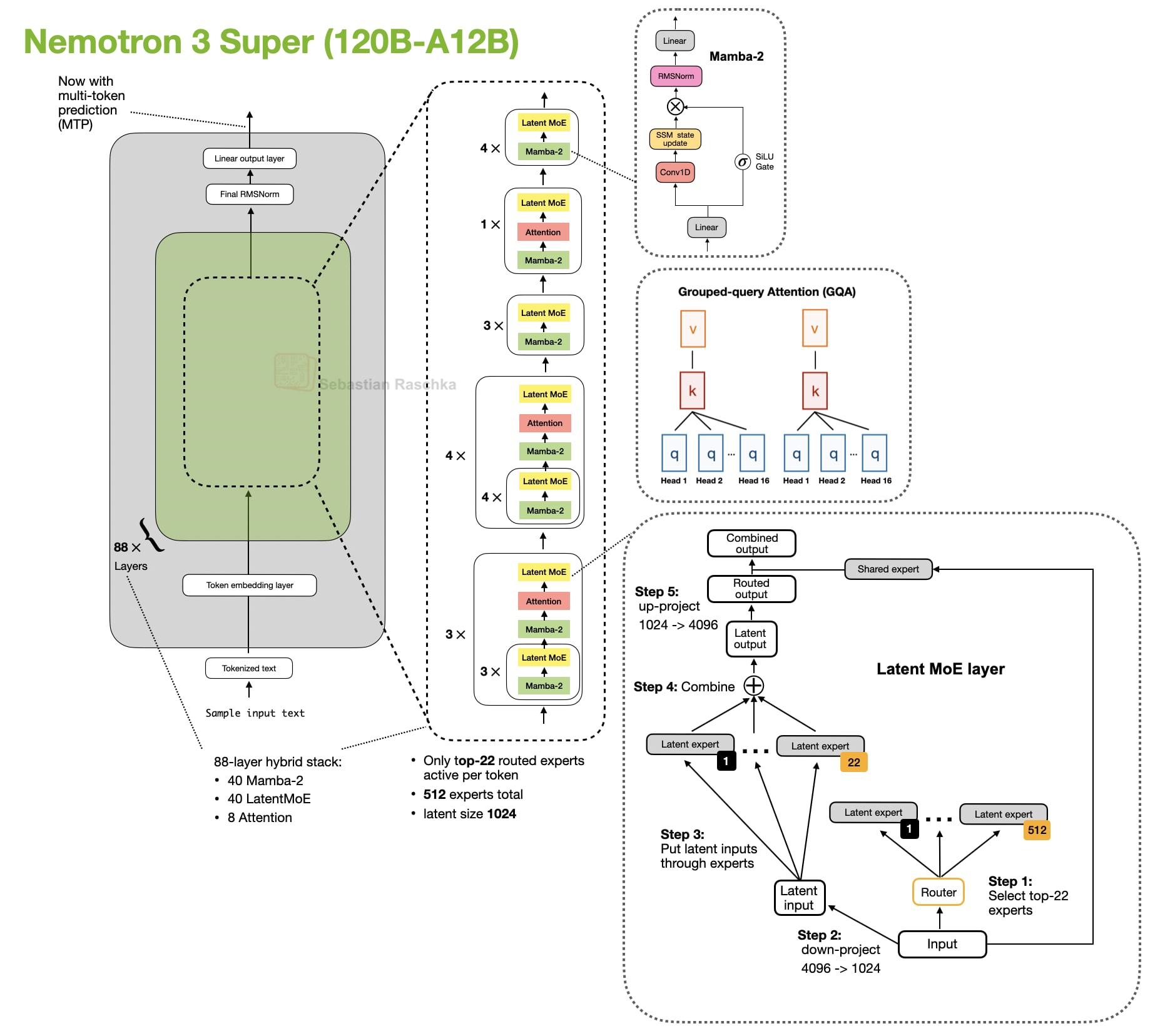
The larger Nemotron 3 Super keeps the Mamba-2 hybrid attention approach and adds other efficiency-oriented changes such as latent MoE and shared-weight multi-token prediction (MTP) for speculative decoding.
Figure 31: Nemotron 3 Super keeps the Mamba-2 hybrid attention pattern while adding latent MoE and shared-weight MTP on top (Original source The Big LLM Architecture Comparison).
Conclusion
Of course, there are many more (mostly niche) attention variants throughout the literature that I haven’t covered here. The focus of this article was on those that are currently used in state-of-the-art (open-weight) models.
In particular, I am looking forward to (1) seeing the brand new Mamba-3 layers getting integrated into the aforementioned hybrid architectures (replacing Gated DeltaNet) and (2) attention residuals being used in general.
In practice, you may also wonder what the “best” architecture is at the moment. This is hard to answer, as there are no public experiments that train different architectures on the same training data etc.
Hence, we can currently only answer what the best (trained) model choice is for a given problem. In my opinion, hybrid architectures are still a novelty, and the main selling point is mainly (long-context) efficiency versus just modeling performance. Hence, I think they are a great candidate for agent contexts (like OpenClaw).
Personally, I think the problem with hybrid architectures is also that the inference stacks are not quite as optimized, yet, and I find that I get better tok/sec throughput when running LLMs locally using more classic setups like GPT-OSS with grouped-query attention.
Anyways, I am curious to see what DeepSeek V4 has in store, since DeepSeek has been quite the reliable trend-setter in the recent 2 years.
Cryptographic encryption algorithms are mathematical procedures that transform readable data into ciphertext that looks like a stream of random bits. The ciphertext can be decrypted only with the corresponding decryption algorithm and the correct key. For data at rest — information stored on disks or in databases — algorithms like AES-XTS encrypt each block before it’s written to storage, protecting against physical theft or unauthorized access to storage systems. For data in transit — information traveling across networks — protocols like TLS combine multiple algorithms: asymmetric encryption algorithms (RSA or elliptic curves) establish secure connections, while fast symmetric encryption algorithms (like AES-GCM) protect the actual data stream and verify that it hasn't been tampered with. At Amazon Web Services (AWS), we use AES-XTS to protect customer data in services like EBS, Nitro cards, and DynamoDB, while TLS with AES-GCM secures all network communication between services and to customers. We took on the challenge of formally verifying an optimized Arm64 assembly implementation of AES-XTS decryption, where “formal verification” is the process of proving mathematically that an engineered system meets a particular specification. Our work follows the IEEE Standard 1619 for cryptographic protection of block-oriented storage devices and focuses on the AES-256-XTS variant of AES-XTS. The “256” specifies the size of the encryption key. Unlike algorithms that process fixed-size blocks, AES-XTS handles variable-length data from 16 bytes up to 16 megabytes, with special logic for incomplete blocks. The assembly code verified was a 5x-unrolled version, meaning that its loops were executed in parallel across five registers (each containing an input block), and it had been optimized for modern CPU pipelines. It was complex enough that manual review couldn't guarantee correctness yet critical enough that errors could compromise customer data security. As part of Amazon Web Services’ s2n-bignum library of formally verified big-number operations, we contributed an improved Arm64 assembly implementation of AES-XTS encryption and decryption, as well as specification and formal verification using the HOL Light interactive theorem prover, which was developed by a member of our team (John Harrison). This was an experiment in the proof-driven development of a large function with multiple paths based on the input length. It resulted in the largest proof so far in the s2n-bignum library. For the typical input size of 512 bytes, the performance of the algorithm either stayed close to that of original code or improved slightly on highly optimized Arm cores. By adding this algorithm and its proof to the s2n-bignum library, we pave the way for more AES-based algorithms to be added. Description of the algorithm AES is a block cipher that implements a keyed permutation. This means that it processes the plaintext files in blocks (in this case, blocks of 128 bits), and for any given key, it defines a bijective (one-to-one and invertible) function mapping each plaintext block to a unique ciphertext block. This mathematical property ensures that decryption can uniquely recover the original plaintext. AES-XTS is the mode specifically designed for storage encryption. It uses AES as its underlying building block but adds position-dependent tweaks and ciphertext stealing — a method for handling partial blocks — to address the unique requirements of disk encryption, where you need random access to any sector and must preserve the exact data size. AES-XTS encrypts storage data using a two-key approach where each 128-bit block and its position-dependent tweak are subjected to an exclusive-OR operation (XOR), a binary operation that outputs a one only if the input values differ. The result of the operation is encrypted with AES, then XORed with the tweak again, ensuring that identical data at different disk locations produces different ciphertext. The tweak is generated by encrypting the sector number with a second key, then multiplying by powers of α in a Galois field, creating unique values for each block position. When the final block isn't a full 128 bits, ciphertext stealing kicks in. Ciphertext stealing borrows bytes from the previous block, allowing encryption of data of any length without padding or wasted space. This lets you read or write any sector independently — critical for disk encryption — while basing each block's encryption on its position. That is a desired feature since the security model of disk encryption allows the adversary to access sectors other than those in question, modify them, and request their decryption. It also ensures that the size of the ciphertext is exactly the same as that of the plaintext, so it fits in its place. Control flow of the assembly implementation We started from an existing implementation of AES-XTS in Amazon’s AWS-LC cryptographic library. AES-XTS loops through the plaintext in 128-bit blocks, and encryption of each block requires 15 steps, each with its own “round key” derived from the encryption key. The existing implementation is 5x unrolled, meaning it processes blocks in parallel, five at a time. If the final block is less than 128 bits in length, there’s a risk of “buffer overread”, or reading beyond the limits of the input buffer. To avoid overread, the existing implementation does complex manipulation over the pointer to the current location in the input buffer. This requires a sophisticated control flow that can be hard to follow: the loop counter is incremented and decremented multiple times before and during the loop, and the loop has two additional exit points other than the final loop-back branch. One exit point is for the case when four blocks remain during the final iteration of the loop; the other exit point is for the case of one to three blocks remaining. The flow of the loop interleaves the load/store instructions with the AES and XOR instructions in an effort to maximize pipeline usage. After the loop exit, the processing of the remaining blocks is intertwined for the lengths of four down to one; if there’s a partial block at the end, the algorithm performs the ciphertext-stealing procedure. Additionally, only seven of the 15 rounds’ keys were kept in registers; the other eight were repeatedly loaded from memory in the loop and outside it. We first investigated whether we could improve the performance of the main loop by letting SLOTHY, a superoptimizer for Arm code, rearrange the instructions to maximize pipeline usage. SLOTHY contains simplified models of various Arm microarchitectures. It uses a constraint solver to provide optimal instruction schedule, register renaming, and periodic loop interleaving. However, for SLOTHY to identify and optimize a loop, the loop has to exhibit typical loop behavior, decreasing the counter at the end of each iteration and then jumping back to the beginning. SLOTHY also cannot handle the nested loop created by loading the eight-round keys. This gave us a reason to start “cleaning up” the loop. First, we freed up registers to permanently hold all round keys; this was possible as the optimized order of instructions required fewer temporary registers than the original code. Second, we removed the multiple exit points and the manipulation of the loop counter to handle the remaining blocks. The value of the counter always indicates the number of five-block chunks remaining in the buffer, conforming to SLOTHY’s requirement; the loop ends before the handling of the remaining blocks. Once the loop ends, we have a separate processing branch to handle each possible number of remaining blocks, from one to four; all four branches end in ciphertext stealing. This can be seen in the control flow graphs of the encrypt and decrypt algorithms (see below). Throughout the code, we maintained the constant-time design mindset; that is, branching and special processing are based not on secret data but only on public values, the input byte lengths. Performance With our modifications to the code, we were able to use SLOTHY to optimize the encrypt algorithm. This resulted in slight performance gains on the AWS Graviton family of Arm processors, although the gains were smaller on the more advanced chips, which have an optimized out-of-order pipeline. Compared to the original implementation, keeping round keys in registers throughout the algorithm’s execution, to save on loading them from memory, allowed us to offset the effects of not interleaving the AES instructions with other ones. Having a cleaner flow of instructions in the loop and modular exit processing allowed us to experiment with various unrolling factors for the loop iterations. We experimented with 3x, 4x, and 6x factors and concluded that 5x is still the best choice across various microarchitectures. Ensuring correctness through formal verification To deploy optimized cryptographic code in production, we need mathematical certainty that it works correctly. While random testing quickly checks simple cases, we rely on formal verification to deliver the highest level of assurance for our AES-XTS implementation. Why HOL Light for AES-XTS? To prove that our implementation matches the IEEE 1619 specification, we use HOL Light, an interactive theorem prover developed by our colleague John Harrison. HOL Light is a particularly simple implementation of the "correct by construction" approach to software development, in which code is verified as it’s written. HOL Light’s trusted kernel is just a few hundred lines of code, which implements basic logical inference rules. This means that even if there's a bug in our proof tactics or automation, it cannot cause HOL Light to accept an incorrect proof. At worst, a bug prevents us from completing a proof, but it cannot make a false statement provable. We chose HOL Light for several reasons specific to AES-XTS verification: Assembly-level verification: We write our implementations directly in assembly rather than relying on compiled code. While more challenging, this makes our proofs independent of any compiler. HOL Light reasons directly about machine code bytes using CPU instruction specifications, providing assurance at the lowest level of the software stack. Existing cryptographic infrastructure: S2n-bignum already provides extensive support for cryptographic verification, including symbolic simulation that strips away execution artifacts and leaves purely mathematical problems, specialized tactics for word operations, and byte list handling. We add proven lemmas about AES operations that we can reuse for the proofs of other AES modes. Complex control flow handling: Unlike fully automated provers that might fail on complex proofs without enough explanation, HOL Light's interactive approach lets us guide proofs through the intricate invariants required for our 5x-unrolled loops, processing arbitrarily long blocks of data and performing the complex memory reasoning required by variable-length inputs and partial blocks. The s2n-bignum framework Using s2n-bignum to implement AES-XTS serves two purposes: it's both a framework for formally verifying assembly code in x86-64 and Arm architectures and a collection of fast, verified assembly functions for cryptography. The library already contains verified implementations of numerous cryptographic algorithms, especially those pertaining to big-number mathematical operations (hence the name), which are the foundation of public-key cryptographic primitives. For details on how HOL Light was used to prove public-key algorithms as part of s2n-bignum, please refer to the previous Amazon Science blog posts “ Formal verification makes RSA faster — and faster to deploy” and “Better-performing ‘25519’ elliptic-curve cryptography”. As we mentioned, AES-XTS is one of the modes of the AES block cipher. AES is based on a substitution-permutation network (SPN) structure, which combines substitution operations (SubBytes using the S-box), permutation operations (ShiftRows, MixColumns), and key mixing. By expanding s2n-bignum to include the AES instruction set architecture (ISA) found in Arm64 and x86_64 processors, specifications for the AES block cipher, and additional specifications for AES-XTS, we're paving the way for the same rigorous verification of more AES-based algorithms. Developing and testing the specification The SPN nature of AES and the modes that are based on it cannot be expressed using simple mathematical formulae — such as modular multiplication, which is fundamental to public-key cryptography — that can be innately understood by a theorem prover. They require writing descriptions of the steps for processing the data. This is why, before verifying the assembly, we needed confidence that our HOL Light specification accurately captured the IEEE standard. We wrote the specification to mirror the standard's structure, using byte lists for input/output and 128-bit words for internal block operations. Then we developed conversions, HOL Light functions that we used to evaluate specifications with concrete inputs while generating proofs that the evaluations are mathematically correct. We validated our specification by conducting unit tests that cover different AES-XTS encryption/decryption scenarios, exercising the processing of all blocks (using recursion) and ciphertext stealing. These tests confirmed that our specification matched the IEEE standard before we tackled the more complex assembly verification. This two-phase approach — first ensuring that the specification is correct through testing, then formally verifying that the implementation matches the specification — gave us confidence we were proving the right thing. The proof strategy Our proofs are compositional, meaning they break the overall problem into subproblems that can be proved separately. Depending on the subproblem, the subproofs can be bounded — true only for a range of inputs — or unbounded. For inputs with fewer than five (or six, in the case of decrypt) blocks, we wrote bounded proofs that exhaustively verify each case. For inputs with five (six, in the case of decrypt) or more blocks, we developed loop invariants — mathematical statements that remain true throughout loop execution — to prove correctness for arbitrarily long inputs. The loop invariants track three critical factors until the loop exit condition is met: register states at each iteration, the evolution of "tweaks" (which make each block's encryption unique), and memory contents as blocks are processed. For partial-block (tail) handling, we proved a separate theorem for ciphertext stealing that could be reused across all cases. The top-level correctness theorem composes all proofs together, asserting the following statement: Memory safety and constant-time proofs Most recently, s2n-bignum was equipped with new functions and tactics for formally defining the constant-time and memory safety properties of assembly functions. With these resources, many assembly subroutines in s2n-bignum were verified to be constant time and memory safe, including top-level scalar-multiplication functions in elliptic curves, big-integer arithmetic for RSA, and the Arm implementation of the ML-KEM cryptography standard (the subject of a forthcoming blog post on Amazon Science). All assembly subroutines identified for use in AWS-LC as of October 2025 were formally verified to be constant time and memory safe. We are exploring whether the new tactics can easily be used to verify assembly subroutines that have subsequently been added, such as AES-XTS. As we mentioned, AES-XTS has a remarkably complex control flow, which resulted in a long and involved functional-correctness proof. That complexity is also a challenge for safety proofs. The process is ongoing, but we have already proved safety properties for the ciphertext-stealing subroutines of the decryption and encryption algorithms. These first proofs focused on crucial memory access procedures that are prone to buffer overread. Proofs for the remaining parts of the decryption and encryption algorithms can use the same methodology, where the constant-time and memory-safety proofs follow the same structure as the functional-correctness proofs but are simpler, since their proof goal is more focused. Continuous assurance of correctness We've integrated formal verification into s2n-bignum's continuous-integration (CI) workflow. This provides assurance that no changes to our AES-XTS implementation can be committed without successfully passing a formal proof of correctness. As part of CI, the CPU instruction modeling is validated through randomized testing against real hardware, "fuzzing out" inaccuracies to ensure our specifications are correct and the proofs hold in practice. Furthermore, the proof guarantees correctness for all possible inputs, since they’re represented in the proof as symbols. This overcomes the typical shortcoming of coverage testing, which may cover all paths of the code but may not be able to cover all input values. For example, a constant-time code, like the one used here, is written without branching on secret values. Typically, then, secret values are incorporated into the operation through the use of masks derived from them. The same instructions are executed irrespective of the secret value. Hence, achieving line coverage is usually within the reach of a developer, but achieving value coverage is left to the formal verification of correctness. This same methodology has enabled AWS to deploy optimized cryptographic implementations with mathematical guarantees of correctness while achieving significant performance improvements. This allows the developer and tools to further optimize the code freely without worrying about introducing bugs, since these will be automatically caught by the proof. Our experience with AES-XTS shows that proof-driven development of assembly code yields a control flow that is easier to understand, review, maintain, and optimize while never ceasing to be provably correct.
Was this newsletter forwarded to you?Sign up to get it in your inbox.
At 4 a.m. on the day after we launched our agent-native document editor, Proof, I watched yet another Codex agent try to revive our server.
Over 4,000 documents had been created since launch, but the app had been mysteriously crashing all day. This left users with crucial documents that they couldn’t access, and me with egg on my face.
I hadn’t slept for almost 24 hours, and all I could do was nervously munch trail mix as Codex investigated yet another bug buried deep in a codebase that I didn’t understand. It felt less like programming and more like being the dumbest participant at a math Olympiad. Needless to say, I was reconsidering my life choices.
Today, almost a week later, Proof is more or less stable. And I’ve learned a lot about both building and launching a purely vibe coded app. Perhaps more importantly, I’ve also learned what happens once that app goes live—and then goes down.
My current opinion is this: If you can vibe code it, you can vibe fix it. You just might not be able to fix it quickly.
Software engineering is changing rapidly as a discipline. The days of typing code into a computer manually seem to be over, and the current conversation on X is around “zero-human startups.” My experience with Proof, though, is a good reality check.
It demonstrates both what is truly possible with vibe coded apps, and where human engineers will continue to be critical now and in the future.
What’s possible at the edge
I’ve been writing about how AI is changing programming for a few years now, and my experience with Proof confirms a lot of my thoughts...
Fine-tuning a large language model (LLM) on a specific task requires updates to billions of parameters across trillions of tokens, with the attendant costs in GPU resources and time. Low-rank adaptation (LoRA) is a more efficient alternative that freezes the original model weights but introduces lightweight matrices into specific model sublayers, or “modules”. These matrices (commonly referred to as “adapters”) modify the modules’ weights, enabling not only efficient fine tuning but also on-demand model serving, which dramatically lowers inference costs; base-model sharing across GPUs, which cuts memory requirements; lower download overhead; and parallel inference across multiple adapters. The question is where to insert these adapters across the model. Empirically, targeting more and larger modules tends to boost performance, because it allows more flexibility in customization; but it also increases training and inference costs. Using a smaller, well-chosen subset preserves most gains with significantly better efficiency. Using Amazon’s Nova 2.0 Lite multimodal reasoning LLM as our base model, we set ourselves the goal of identifying a subset of standardized target-module configurations that works effectively across the vast majority of customer use cases. Through an ablation study, we identified a module known as o_proj, as the single module where adding an adapter achieves the best trade-off between efficiency and accuracy (o_proj is a linear transformation that mixes representations across attention heads into a single, cohesive form for the rest of the model to understand). The Transformer architecture Transformer models — the models responsible for all of AI’s remarkable recent gains — consist largely of blocks that are repeated multiple times. Each block in turn has two main components: an attention mechanism, which determines the relevance of previously seen tokens to the token currently being processed, and a feed-forward network, a conventional neural network that does additional processing on the outputs of the attention mechanism. The attention mechanism involves three different matrices, which take their names from database design: the query matrix represents how relevant the current token is to the other tokens in the input sequence; the key matrix represents how relevant other tokens are to one another; and the value matrix represents the raw content of those other tokens. Multiplying the three matrices together creates, essentially, a recipe for the Transformer's next output. To reduce computational complexity, these multiplications take place in a space with reduced dimensions. The matrices themselves and the results of their multiplication then have to be projected back up to the original dimensions of the input. LoRA approximates weight updates using a product of two smaller matrices, drastically reducing the number of trainable parameters. The technique is typically applied to attention projection layers and feed-forward network layers. These modules are ideal candidates because they constitute the bulk of Transformer parameters, directly govern representation learning, and exhibit natural alignment with low-rank approximations. Empirical evidence shows weight changes in these layers often lie within a low-dimensional subspace during fine tuning. Target module selection Selecting the right target modules directly affects accuracy, latency, and computational efficiency. The optimal choice of target modules is primarily a function of (a) the base model being fine-tuned (i.e., its architecture, pre- and post-training data distributions, etc.) and (b) customization domain/modality. When fine-tuning Nova 2.0 Lite, we balanced two competing objectives: Maximizing accuracy across diverse tasks and modalities and Minimizing latency to preserve LoRA's efficiency benefits. We investigated the application of LoRA to four different modules in each Transformer block: the query, key, and value projection layers ( qkv); the o_proj layer; and two different fully connected layers in the feed-forward network, gate_up_proj and gate_down_proj (referred to as fc1 and fc2). Below are the trade-offs for these modules, both singly and in combination, based on results published in literature and empirical studies. CombinationExpected accuracyExpected latencyUse caseqkv onlyGood (baseline)Lowest Resource-constrained environments Tasks where attention mechanisms are critical (e.g., classification, lightweight generation) Prioritizes speed over maximum accuracy o_proj onlyModerateLowest Ultralow-latency scenarios Tasks where refining attention outputs is sufficient (e.g., simple sentiment analysis). Plays an important role in reasoning Less effective than qkv, but very efficient qkv + o_projHighLow to moderate (+5–10%) Attention-focused tasks (e.g., machine translation, summarization) Balances refinement of both attention context ( o_proj) and query/key/value projections ( qkv) Best accuracy-to-latency ratio for most NLP tasks qkv + fc1 / fc2Very high (close to full fine tuning)Moderate (+10–15%) Complex generation tasks (e.g., translation, long-form summarization) When feed-forward layers ( fc1/ fc2) significantly influence output quality as they store and retrieve factual knowledge Prioritizes accuracy over speed o_proj + fc1 / fc2Good to highModerate (+5–10%) Tasks requiring adaptation of both attention output ( o_proj) and feed-forward layers (e.g., text classification, sentiment analysis) Suitable when qkv adaptation is unnecessary qkv + o_proj + fc1 / fc2Highest (near-full fine tuning)High (+15–20%) Maximum accuracy for critical tasks (e.g., research benchmarks, high-stakes generation) When all components of the Transformer block need adaptation Avoid for production if latency matters All modules ( qkv, o_proj, fc1, fc2)MaximumHighest (+20–25%) Prototyping/research with no latency constraints Rarely justified in practice; marginal gains over qkv + o_proj + fc1/ fc2 Trade-offs of accuracy and latency across target modules, based on literature review and empirical evidence. Experimental methodology We conducted a comprehensive ablation study, training multiple supervised-fine-tuning (SFT) LoRA variants on seven datasets spanning both text and visual data, across reasoning (i.e., the training datasets themselves include reasoning content) and non-reasoning tasks. The datasets covered diverse challenges from simple question answering to long-context summarization and structured JSON extraction. DatasetModalityReasoning tracesDomainTasksTraining sizeEval sizeEval metricSourceFinCOTTxtYesFinanceFinancial-reasoning dataset. Samples consist of complex financial queries, along with reasoning traces obtained from GPT-4o. Predictions are typically complex tables or calculations based on the input.74361147Accuracyhttps://huggingface.co/datasets/TheFinAI/FinCoTGovReportTxtNoGoverment DocLarge-context (30-40K tokens) summarization17457837RougeLsumhttps://gov-report-data.github.io/MedMCQATxtNoMedicalDataset for multiple-choice QA — also used in Nova 1.020k3683Accuracyhttps://huggingface.co/datasets/openlifescienceai/medmcqaMedReasonTxtYesMedicalMedical-reasoning dataset that consists of questions and answers compiled from various medical benchmarks (MedQA, MedMCQA, etc.), along with synthetic, high-quality reasoning traces. (This uses the same eval set as MedMCQA.)316823683Accuracyhttps://huggingface.co/datasets/UCSC-VLAA/MedReasonCoCoHDTxtNoPolitical DocA complex benchmark consisting of large-context (>20K tokens) transcripts of congressional hearings. The output is expected to be a summary in a specific JSON format, consisting of the members present, topic discussed, outcomes, etc.7321053Averaged key and value match ratehttps://github.com/gtfintechlab/CoCoHDLlava-COTImageYesImage understanding, General/ScienceMultimodal, image benchmark consisting of Q&A reasoning questions. The dataset includes high-quality reasoning traces.10k270Exact match ratehttps://huggingface.co/datasets/Xkev/LLaVA-CoT-100kInvoice OCRImageNoImage understandingOCR benchmark that takes an input image and produces a JSON file with fields from the image.1400447AccuracySummary of the experiment datasets All experiments used the Nova 2.0 Lite general-availability checkpoint with consistent hyperparameters across target modules, including learning-rate ratio and alpha values. Target datasetSettingSFT LoRA target performanceNova 2.0 Lite performanceFin-COTqkv67.09%72.12%o_proj68.30%fc175.35%fc260.24%o_proj + fc161.38%qkv + fc260.31%o_proj + fc262.79%qkv + fc168.37%All target modules66.15%CoCoHDqkv19.64%45.14%o_proj65.88%fc141.96%fc217.62%o_proj + fc176.83%qkv + fc266.47%o_proj + fc279.14%qkv + fc145.45%All target modules82.75%GovReporto_proj41.25%38.90%fc139.69%o_proj + fc141.74%o_proj + fc242.16%qkv + fc141.66%qkv + fc239.02%All target modules41.95%Llava-COTqkv64.26%16.22%o_proj64.26%fc165.92%fc265.02%o_proj + fc163.21%qkv + fc262.76%o_proj + fc266.37%qkv + fc166.52%All target modules63.96%Invoice OCRo_proj89.07%14.10%o_proj + fc190.03%qkv + fc287.84%o_proj + fc289.47%qkv + fc188.55%All target modules90.11%MedReasono_proj24.55%1.68%o_proj + fc120.88%qkv + fc28.39%o_proj + fc220.36%qkv + fc14.32%All target modules26.72%MedMCQAqkv62.18%1.68%o_proj63.10%fc112.90%fc259.98%o_proj + fc161.39%qkv + fc265.63%o_proj + fc264.95%qkv + fc157.21%All target modules66.11%Ablation study for target module selection. Some benchmarks have fewer variations, to save on computation and time. MedMCQA and MedReason use the MedMCQA test set for evaluation. On this task, Nova 2.0 Lite fails mainly due to formatting inconsistencies, even though it produces the right answer. For consistency’s sake, we use the same strict parser for SFT models. Key findings 1. O_proj is the most robust single target The o_proj-only configuration demonstrated remarkable consistency, never failing outright on any task and typically performing within a few percentage points of the best configuration (i.e., using all target modules). On MedMCQA, CoCoHD, GovReport, LLaVA-CoT, and Invoice OCR, o_proj-only either matched or came very close to optimal performance, making it an attractive default choice that balances performance and simplicity. There is emerging evidence that this module plays a key role in reasoning, which may explain its effectiveness here. 2. Qkv-only shows instability While qkv-only performed well on MedMCQA, it exhibited extreme variability, performing below baseline on CoCoHD and showing unremarkable results elsewhere. This aligns with the hypothesis that attention-only LoRA can underfit on tasks requiring richer features from the feed-forward network, rather than relying on modified token routing. 3. Module combinations provide modest gains Combinations like o_proj + fc2 or "all target modules" often achieved the highest per-dataset scores (particularly on CoCoHD, MedReason, and Invoice OCR). However, improvements over the best single module were typically modest, usually 1-3 percentage points. 4. Task difficulty amplifies configuration impact On challenging benchmarks where the base model performed poorly, the choice of target modules had greater impact. For example, on CoCoHD (long-context, complex JSON generation), o_proj + fc2 achieved a +15% absolute improvement over the base model, compared to only +3% with o_proj alone. 5. LoRA consistently outperforms base models Across nearly all datasets, any reasonable LoRA configuration dramatically outperformed the base model. For instance, MedReason, MedMCQA, LLaVA-CoT, and Invoice OCR showed improvements from a baseline accuracy of ~1-16% to 60-90%+ with LoRA. The notable exception was Fin-COT, where only certain configurations (notably fc1) exceeded baseline performance, suggesting task-specific sensitivity to adaptation strategy. Recommendations For accuracy-prioritized scenarios, we recommend o_proj + fc2 as the optimal configuration for both text and multimodal tasks, showing 2-12% improvements over o_proj alone across benchmarks. For balanced efficiency and performance, o_proj-only provides an excellent default, offering robust performance with minimal latency overhead — particularly valuable when serving multiple adapters or operating under resource constraints. For challenging tasks, such as benchmarks with long context or complex generation requirements or other tasks where base models struggle, the additional accuracy from o_proj + fc2 justifies the modest latency increase. Future directions Our research opens several promising avenues for further optimization: Modality and task-specific configurations: Segmenting target module selection by modality and task difficulty (e.g., long-context scenarios) could yield specialized configurations with better accuracy-latency trade-offs. Per-module hyperparameter optimization: Extensive hyperparameter optimization for each target module configuration could unlock additional performance gains, though computational costs remain a consideration. Two-stage LoRA for early candidate identification: Leveraging two-stage LoRA approaches that use training dynamics, gradients, etc., to determine the importance of different modules/layers could help identify promising configurations early in training, reducing the cost of comprehensive hyperparameter searches. Layer pruning for latency reduction: Using two-stage training to identify and prune unused layers could further reduce inference latency while maintaining accuracy. Conclusion Our comprehensive study demonstrates that thoughtful target module selection in LoRA fine tuning can improve accuracy while preserving the efficiency advantages that make LoRA attractive for production deployments. The o_proj layer emerges as a remarkably robust single target, while o_proj + fc2 combinations offer the best accuracy for challenging tasks. On average, o_proj LoRA is within 2% of o_proj + fc2 in terms of accuracy but has 22.6% lower latency (TPOT p95 decreases from 10.085ms → 7.803ms). These findings provide a principled foundation for standardizing LoRA configurations across diverse customer use cases, balancing the competing demands of model performance and computational efficiency. Acknowledgements: Kevin Rondinone, Kevin Chen, Nicole Ding, Sebastian Massella, Andy Li

 Login
Login