 Login
LoginQIMMA قِمّة ⛰: A Quality-First Arabic LLM Leaderboard
21 April 2026 at 10:09



GRASP is a new gradient-based planner for learned dynamics (a “world model”) that makes long-horizon planning practical by (1) lifting the trajectory into virtual states so optimization is parallel across time, (2) adding stochasticity directly to the state iterates for exploration, and (3) reshaping gradients so actions get clean signals while we avoid brittle “state-input” gradients through high-dimensional vision models.
Large, learned world models are becoming increasingly capable. They can predict long sequences of future observations in high-dimensional visual spaces and generalize across tasks in ways that were difficult to imagine a few years ago. As these models scale, they start to look less like task-specific predictors and more like general-purpose simulators.
But having a powerful predictive model is not the same as being able to use it effectively for control/learning/planning. In practice, long-horizon planning with modern world models remains fragile: optimization becomes ill-conditioned, non-greedy structure creates bad local minima, and high-dimensional latent spaces introduce subtle failure modes.
In this blog post, I describe the problems that motivated this project and our approach to address them: why planning with modern world models can be surprisingly fragile, why long horizons are the real stress test, and what we changed to make gradient-based planning much more robust.
This blog post discusses work done with Mike Rabbat, Aditi Krishnapriyan, Yann LeCun, and Amir Bar (* denotes equal advisorship), where we propose GRASP.
These days, the term “world model” is quite overloaded, and depending on the context can either mean an explicit dynamics model or some implicit, reliable internal state that a generative model relies on (e.g. when an LLM generates chess moves, whether there is some internal representation of the board). We give our loose working definition below.
Suppose you take actions $a_t \in \mathcal{A}$ and observe states $s_t \in \mathcal{S}$ (images, latent vectors, proprioception). A world model is a learned model that, given the current state and a sequence of future actions, predicts what will happen next. Formally, it defines a predictive distribution on a sequence of observed states $s_{t-h:t}$ and current action $a_t$:
\[P_\theta(s_{t+1} \mid s_{t-h:t},\; a_t)\]that approximates the environment’s true conditional $P(s_{t+1} \mid s_{t-h:t},\; a_t)$. For this blog post, we’ll assume a Markovian model $P(s_{t+1} \mid s_{t-h:t},\; a_t)$ for simplicity (all results here can be extended to the more general case), and when the model is deterministic it reduces to a map over states:
\[s_{t+1} = F_\theta(s_t, a_t).\]In practice the state $s_t$ is often a learned latent representation (e.g., encoded from pixels), so the model operates in a (theoretically) compact, differentiable space. The key point is that a world model gives you a differentiable simulator; you can roll it forward under hypothetical action sequences and backpropagate through the predictions.
Given a start $s_0$ and a goal $g$, the simplest planner chooses an action sequence $\mathbf{a}=(a_0,\dots,a_{T-1})$ by rolling out the model and minimizing terminal error:
\[\min_{\mathbf{a}} \; \| s_T(\mathbf{a}) - g \|_2^2, \quad \text{where } s_T(\mathbf{a}) = \mathcal{F}_{\theta}^{T}(s_0,\mathbf{a}).\]Here we use $\mathcal{F}^T$ as shorthand for the full rollout through the world model (dependence on model parameters $\theta$ is implicit):
\[\mathcal{F}_{\theta}^{T}(s_0, \mathbf{a}) = F_\theta(F_\theta(\cdots F_\theta(s_0, a_0), \cdots, a_{T-2}), a_{T-1}).\]In short horizons and low-dimensional systems, this can work reasonably well. But as horizons grow and models become larger and more expressive, its weaknesses become amplified.
So why doesn’t this just work at scale?
There are two separate pain points for the more general world model, plus a third that is specific to learned, deep learning-based models.
Those familiar with backprop through time (BPTT) may notice that we’re differentiating through a model applied to itself repeatedly, which will lead to the exploding/vanishing gradients problem. Namely, if we take derivatives (note we’re differentiating vector-valued functions, resulting in Jacobians that we denote with $D_x (\cdots)$) with respect to earlier actions (e.g. $a_0$):
\[D_{a_0} \mathcal{F}_{\theta}^{T}(s_0, \mathbf{a}) = \Bigl(\prod_{t=1}^T D_s F_\theta(s_t, a_t)\Bigr) D_{a_0}F_\theta(s_0, a_0).\]We see that the Jacobian’s conditioning scales exponentially with time $T$:
\[\sigma_{\text{max/min}}(D_{a_0}\mathcal{F}_{\theta}^{T}) \sim \sigma_{\text{max/min}}(D_s F_\theta)^{T-1},\]leading to exploding or vanishing gradients.
At short horizons, the greedy solution, where we move straight toward the goal at every step, is often good enough. If you only need to plan a few steps ahead, the optimal trajectory usually doesn’t deviate much from “head toward $g$” at each step.
As horizons grow, two things happen. First, longer tasks are more likely to require non-greedy behavior: going around a wall, repositioning before pushing, backing up to take a better path. And as horizons grow, more of these non-greedy steps are typically needed. Second, the optimization space itself scales with horizon: $\mathrm{dim}(\mathcal{A} \times \cdots \times \mathcal{A}) = T\mathrm{dim}(\mathcal{A})$, further expanding the space of local minima for the optimization problem.
Suppose we treat the dynamics constraint $s_{t+1} = F_{\theta}(s_t, a_t)$ as a soft constraint, and we instead optimize the following penalty function over both actions $(a_0,\ldots,a_{T-1})$ and states $(s_0,\ldots,s_T)$:
\[\min_{\mathbf{s},\mathbf{a}} \mathcal{L}(\mathbf{s}, \mathbf{a}) = \sum_{t=0}^{T-1} \big\|F_\theta(s_t,a_t) - s_{t+1}\big\|_2^2, \quad \text{with } s_0 \text{ fixed and } s_T=g.\]This is also sometimes called collocation in planning/robotics literature. Note the lifted formulation shares the same global minimizers as the original rollout objective (both are zero exactly when the trajectory is dynamically feasible). But the optimization landscapes are very different, and we get two immediate benefits:
Being able to optimize states directly also helps with exploration, as we can temporarily navigate through unphysical domains to find the optimal plan:
However, lunch is never free. And indeed, especially for deep learning-based world models, there is a critical issue that makes the above optimization quite difficult in practice.
The tl;dr of this section is: directly optimizing states through a deep learning-based $F_{\theta}$ is incredibly brittle, à la adversarial robustness. Even if you train your world model in a lower-dimensional state space, the training process for the world model makes unseen state landscapes very sharp, whether it be an unseen state itself or simply a normal/orthogonal direction to the data manifold.
Adversarial robustness originally looked at classification models $f_\theta : \mathbb{R}^{w\times h \times c} \to \mathbb{R}^K$, and showed that by following the gradient of a particular logit $\nabla f_\theta^k$ from a base image $x$ (not of class $k$), you did not have to move far along $x’ = x + \epsilon\nabla f_\theta^k$ to make $f_\theta$ classify $x’$ as $k$ (Szegedy et al., 2014; Goodfellow et al., 2015):
Later work has painted a geometric picture for what’s going on: for data near a low-dimensional manifold $\mathcal{M}$, the training process controls behavior in tangential directions, but does not regularize behavior in orthogonal directions, thus leading to sensitive behavior (Stutz et al., 2019). Another way stated: $f_\theta$ has a reasonable Lipschitz constant when considering only tangential directions to the data manifold $\mathcal{M}$, but can have very high Lipschitz constants in normal directions. In fact, it often benefits the model to be sharper in these normal directions, so it can fit more complicated functions more precisely.
As a result, such adversarial examples are incredibly common even for a single given model. Further, this is not just a computer vision phenomenon; adversarial examples also appear in LLMs (Wallace et al., 2019) and in RL (Gleave et al., 2019).
While there are methods to train for more adversarially robust models, there is a known trade-off between model performance and adversarial robustness (Tsipras et al., 2019): especially in the presence of many weakly-correlated variables, the model must be sharper to achieve higher performance. Indeed, most modern training algorithms, whether in computer vision or LLMs, do not train adversarial robustness out. Thus, at least until deep learning sees a major regime change, this is a problem we’re stuck with.
Consider a single component of the dynamics loss we’re optimizing in the lifted state approach:
\[\min_{s_t, a_t, s_{t+1}} \|F_\theta(s_t, a_t) - s_{t+1}\|_2^2\]Let’s further focus on just the base state:
\[\min_{s_t} \|F_\theta(s_t, a_t) - s_{t+1}\|_2^2.\]Since world models are typically trained on state/action trajectories $(s_1, a_1, s_2, a_2, \ldots)$, the state-data manifold for $F_{\theta}$ has dimensionality bounded by the action space:
\[\mathrm{dim}(\mathcal{M}_s) \le \mathrm{dim}(\mathcal{A}) + 1 + \mathrm{dim}(\mathcal{R}),\]where $\mathcal{R}$ is some optional space of augmentations (e.g. translations/rotations). Thus, we can typically expect $\mathrm{dim}(\mathcal{M}_s)$ to be much lower than $\mathrm{dim}(\mathcal{S})$, and thus: it is very easy to find adversarial examples that hack any state to any other desired state.
As a result, the dynamics optimization
\[\sum_{t=0}^{T-1} \big\|F_\theta(s_t,a_t) - s_{t+1}\big\|_2^2\]feels incredibly “sticky,” as the base points $s_t$ can easily trick $F_{\theta}$ into thinking it’s already made its local goal.1
1. This adversarial robustness issue, while particularly bad for lifted-state approaches, is not unique to them. Even for serial optimization methods that optimize through the full rollout map $\mathcal{F}^T$, it is possible to get into unseen states, where it is very easy to have a normal component fed into the sensitive normal components of $D_s F_{\theta}$. The action Jacobian’s chain rule expansion is
\[\Bigl(\prod_{t=1}^T D_s F_\theta(s_t, a_t)\Bigr) D_{a_0}F_\theta(s_0, a_0).\]See what happens if any stage of the product has any component normal to the data manifold. ↩
This is where our new planner GRASP comes in. The main observation: while $D_s F_{\theta}$ is untrustworthy and adversarial, the action space is usually low-dimensional and exhaustively trained, so $D_a F_{\theta}$ is actually reasonable to optimize through and doesn’t suffer from the adversarial robustness issue!
At its core, GRASP builds a first-order lifted state / collocation-based planner that is only dependent on action Jacobians through the world model. We thus exploit the differentiability of learned world models $F_{\theta}$, while not falling victim to the inherent sensitivity of the state Jacobians $D_s F_{\theta}$.
As noted before, we start with the collocation planning objective, where we lift the states and relax dynamics into a penalty:
\[\min_{\mathbf{s},\mathbf{a}} \mathcal{L}(\mathbf{s}, \mathbf{a}) = \sum_{t=0}^{T-1} \big\|F_\theta(s_t,a_t) - s_{t+1}\big\|_2^2, \quad \text{with } s_0 \text{ fixed and } s_T=g.\]We then make two key additions.
Even with a smoother objective, planning is nonconvex. We introduce exploration by injecting Gaussian noise into the virtual state updates during optimization.
A simple version:
\[s_t \leftarrow s_t - \eta_s \nabla_{s_t}\mathcal{L} + \sigma_{\text{state}} \xi, \qquad \xi\sim\mathcal{N}(0,I).\]Actions are still updated by non-stochastic descent:
\[a_t \leftarrow a_t - \eta_a \nabla_{a_t}\mathcal{L}.\]The state noise helps you “hop” between basins in the lifted space, while the actions remain guided by gradients. We found that specifically noising states here (as opposed to actions) finds a good balance of exploration and the ability to find sharper minima.2
2. Because we only noise the states (and not the actions), the corresponding dynamics are not truly Langevin dynamics. ↩
As discussed, the fragile pathway is the gradient that flows into the state input of the world model, \(D_s F_{\theta}\). The most straightforward way to do this initially is to just stop state gradients into \(F_{\theta}\) directly:
Define the stop-gradient dynamics loss:
\[\mathcal{L}_{\text{dyn}}^{\text{sg}}(\mathbf{s},\mathbf{a}) = \sum_{t=0}^{T-1} \big\|F_\theta(\bar{s}_t, a_t) - s_{t+1}\big\|_2^2.\]This alone does not work. Notice now states only follow the previous state’s step, without anything forcing the base states to chase the next ones. As a result, there are trivial minima for just stopping at the origin, then only for the final action trying to get to the goal in one step.
We can view the above issue as the goal’s signal being cut off entirely from previous states. One way to fix this is to simply add a dense goal term throughout prediction:
\[\mathcal{L}_{\text{goal}}^{\text{sg}}(\mathbf{s},\mathbf{a}) = \sum_{t=0}^{T-1} \big\|F_\theta(\bar{s}_t, a_t) - g\big\|_2^2.\]In normal settings this would over-bias towards the greedy solution of straight chasing the goal, but this is balanced in our setting by the stop-gradient dynamics loss’s bias towards feasible dynamics. The final objective is then as follows:
\[\mathcal{L}(\mathbf{s},\mathbf{a}) = \mathcal{L}_{\text{dyn}}^{\text{sg}}(\mathbf{s},\mathbf{a}) + \gamma \, \mathcal{L}_{\text{goal}}^{\text{sg}}(\mathbf{s},\mathbf{a}).\]The result is a planning optimization objective that does not have dependence on state gradients.
The lifted stop-gradient objective is great for fast, guided exploration, but it’s still an approximation of the original serial rollout objective.
So every $K_{\text{sync}}$ iterations, GRASP does a short refinement phase:
The lifted-state optimization still provides the core of the optimization, while this refinement step adds some assistance to keep states and actions grounded towards real trajectories. This refinement step can of course be replaced with a serial planner of your choice (e.g. CEM); the core idea is to still get some of the benefit of the full-path synchronization of serial planners, while still mostly using the benefits of the lifted-state planning.
Collocation-based planners offer a natural fix for long-horizon planning, but this optimization is quite difficult through modern world models due to adversarial robustness issues. GRASP proposes a simple solution for a smoother collocation-based planner, alongside stable stochasticity for exploration. As a result, longer-horizon planning ends up not only succeeding more, but also finding such successes faster:
| Horizon | CEM | GD | LatCo | GRASP |
|---|---|---|---|---|
| H=40 | 61.4% / 35.3s | 51.0% / 18.0s | 15.0% / 598.0s | 59.0% / 8.5s |
| H=50 | 30.2% / 96.2s | 37.6% / 76.3s | 4.2% / 1114.7s | 43.4% / 15.2s |
| H=60 | 7.2% / 83.1s | 16.4% / 146.5s | 2.0% / 231.5s | 26.2% / 49.1s |
| H=70 | 7.8% / 156.1s | 12.0% / 103.1s | 0.0% / — | 16.0% / 79.9s |
| H=80 | 2.8% / 132.2s | 6.4% / 161.3s | 0.0% / — | 10.4% / 58.9s |
Push-T results. Success rate (%) / median time to success. Bold = best in row. Note the median success time will bias higher with higher success rate; GRASP manages to be faster despite higher success rate.
There is still plenty of work to be done for modern world model planners. We want to exploit the gradient structure of learned world models, and collocation (lifted-state optimization) is a natural approach for long-horizon planning, but it’s crucial to understand typical gradient structure here: smooth and informative action gradients and brittle state gradients. We view GRASP as an initial iteration for such planners.
Extension to diffusion-based world models (deeper latent timesteps can be viewed as smoothed versions of the world model itself), more sophisticated optimizers and noising strategies, and integrating GRASP into either a closed-loop system or RL policy learning for adaptive long-horizon planning are all natural and interesting next steps.
I do genuinely think it’s an exciting time to be working on world model planners. It’s a funny sweet spot where the background literature (planning and control overall) is incredibly mature and well-developed, but the current setting (pure planning optimization over modern, large-scale world models) is still heavily underexplored. But, once we figure out all the right ideas, world model planners will likely become as commonplace as RL.
For more details, read the full paper or visit the project website.
@article{psenka2026grasp,
  title={Parallel Stochastic Gradient-Based Planning for World Models},
  author={Michael Psenka and Michael Rabbat and Aditi Krishnapriyan and Yann LeCun and Amir Bar},
  year={2026},
  eprint={2602.00475},
  archivePrefix={arXiv},
  primaryClass={cs.LG},
  url={https://arxiv.org/abs/2602.00475}
}
It’s a clear, current equilibrium that open models will be in perpetual catch-up of closed models, but this gap being viewed as a single number, a “distance”, covers up a nuanced and crucial dynamic at what capabilities the models are covering. The most popular benchmark to comment on this gap is the Artificial Analysis Intelligence Index — a composite benchmark of ~10 sub-evals that they maintain over time to capture the “frontier” of current language model capabilities.
Particularly, I spend a lot of time understanding how dynamics that feed into that index are misunderstood by the natural tendency to reduce performance and trends to one number. Examples include:
How benchmarks evolve over time, becoming more or less correlated with how people actually use models,
How different models’ real-world performance relates to their benchmark rankings, and
How training regimes evolve over time to move said benchmarks.
Agentic benchmarks are in a decent place, but benchmarks are no longer as trusted as a correlate to real-world performance. A key example to this gray area is Gemini 3’s incredible benchmarks and remarkable irrelevance in where AI tools currently are being tested and deployed (agents). These trends point to obvious and lasting flaws in our measurements.
At the root of this dynamic — the dance of correlating model real-world performance and benchmark scores — is the constant shift of the industry. As all the models, i.e. both open and closed, evolve over time, the topics of focus for benchmarking shifts about every 12 to 18 months. All of the domains of interest have very different training domains associated with them, especially in post-training. The longer a single paradigm goes on, the better the industry gets at measuring performance. In a new era of rapid post-training improvements, I’m at a relative minimum in my personal confidence in benchmarks.
Right after ChatGPT the focus was a mix of chat, math, and simple code. Instruction tuning and RLHF dominated. Chat capabilities saturated and faded quickly, then mathematics became less focal. Through 2025 and to today, especially once reasoning models became the default, the focus shifted to more complex coding and other simpler agentic tasks. We’re at the tail end of this first era. Recent training recipes are all dominated by reinforcement learning with verifiable rewards (RLVR), but the domains it is applied in have shifted dramatically from basic question-answer checking to complex environments.
What we’re seeing is that the closed, frontier labs are investing astounding sums of money in mastering these current foci — i.e. code, terminal tasks, etc. — while starting to push into more diverse knowledge work tasks. These newer tasks encompass specialized domains, such as accounting, law, healthcare, etc. They are still agentic, but require more expertise and often integrations with existing software or domain-specific tools.
We have very limited evidence on the true balance of capabilities of these newer domains, but these are the areas I’m focusing on when I say open models will struggle to keep up. The problem is that evaluating complex language model workflows is also a challenging research problem in itself.
The tasks are getting harder and the data needed to hillclimb on them is getting more private (relative to code, which has swaths of code on GitHub). Leading open model labs are helped by dynamics happening in the data industry that are economically similar to building chip fabs. The few, leading labs in the U.S. pay astronomical sums to buy new environments and datasets, then the fast-following labs (often in China), buy these later at a steep discount.
This is a key missed point — that the levers non-frontier labs pull to keep up constantly shift over time. A focus on distillation as the key lever to Chinese models’ progress reflects a blind-spot to the importance of RL environments to current training regimes. If an environment can be built either as a single evaluation in the Artificial Analysis Index, or to mirror it, currently the Chinese labs will be able to keep up.
Interconnects AI is a reader-supported publication. Consider becoming a subscriber.
The question worth dwelling on is: How crucial is the current set of tasks (again, coding and terminal tasks), where the likes of OpenAI and Anthropic have a massive business-adoption advantage over leading open weight models (and even Google alike), is crucial to maintaining revenue numbers? In order to maintain these record growth numbers and trajectories, there needs to keep being a meaningful edge in performance. Many companies would love to reduce their token expenditure cost if they can swap in a far cheaper, open model equivalent.
If agentic coding abilities saturate and the “frontier” of AI performance moves elsewhere, a large amount of the enterprise revenue could be reliant on well-formed customer relationships, inertia, and better product development, rather than the models being leaps and bounds better.
This precarious position is what I describe as the frontier labs needing to constantly reinvent themselves, and the field’s prospects, for monetizing the vast buildout of AI infrastructure. I still tend to fall on the side that the buildout will be worth it, and Anthropic and OpenAI will be astronomically profitable businesses, so I take this as a faith of a mix of them continuing to unlock compelling, new, valuable use-cases for the models, and that the benchmarks the open models are closing in on as not being a complete signal.
I operate with a sort of presumption where the leading open models from China are focused slightly more on benchmarks than the leading closed labs in the U.S. They’re incentivized to do so — they want to present the image as constantly being on the heels of the best closed models. Saying the Chinese labs are only in this narrative because they’re overfitting to benchmarks would be incredibly naive and incorrect. They’re genuinely strong models, and these dynamics of overselling and real innovation are a fine balance.
There are a few out-of-distribution benchmarks where open-weight models are very far behind, such as WeirdML or ARC AGI 2, but there are countless random benchmarks that show these open models as being unexpectedly strong. When you use the models, you can pick up on this lack of robustness (e.g. in long-context capabilities, and needing to reset your agent context more often than Claude/Codex), but they’re not a category error in the sense that they’re fundamentally different classes of models. They’re far closer than many would’ve expected.
Many people asked me over the past months to share my workflow for how I come up with the LLM architecture sketches and drawings in my articles, talks, and the LLM-Gallery. So I thought it would be useful to document the process I usually follow.
The short version is that I usually start with the official technical reports, but these days, papers are often less detailed than they used to be, especially for most open-weight models from industry labs.
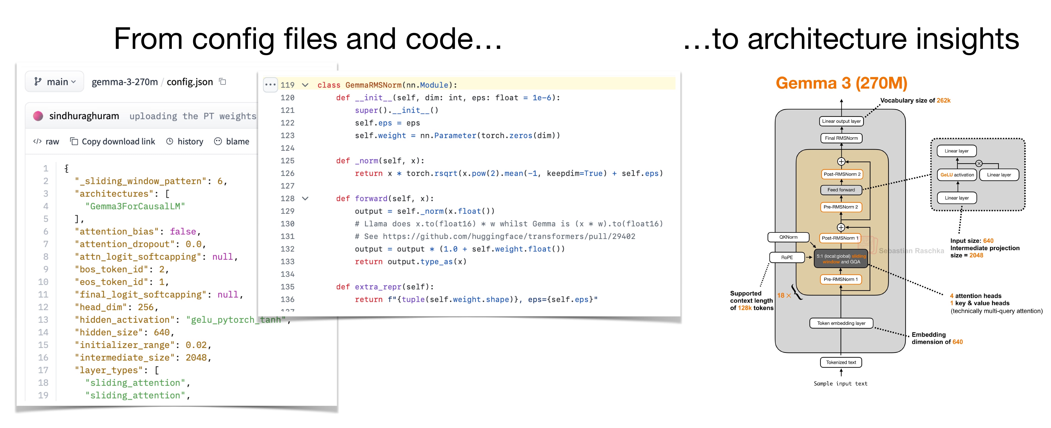
The good part is that if the weights are shared on the Hugging Face Model Hub and the model is supported in the Python transformers library, we can usually inspect the config file and the reference implementation directly to get more information about the architecture details. And “working” code doesn’t lie.
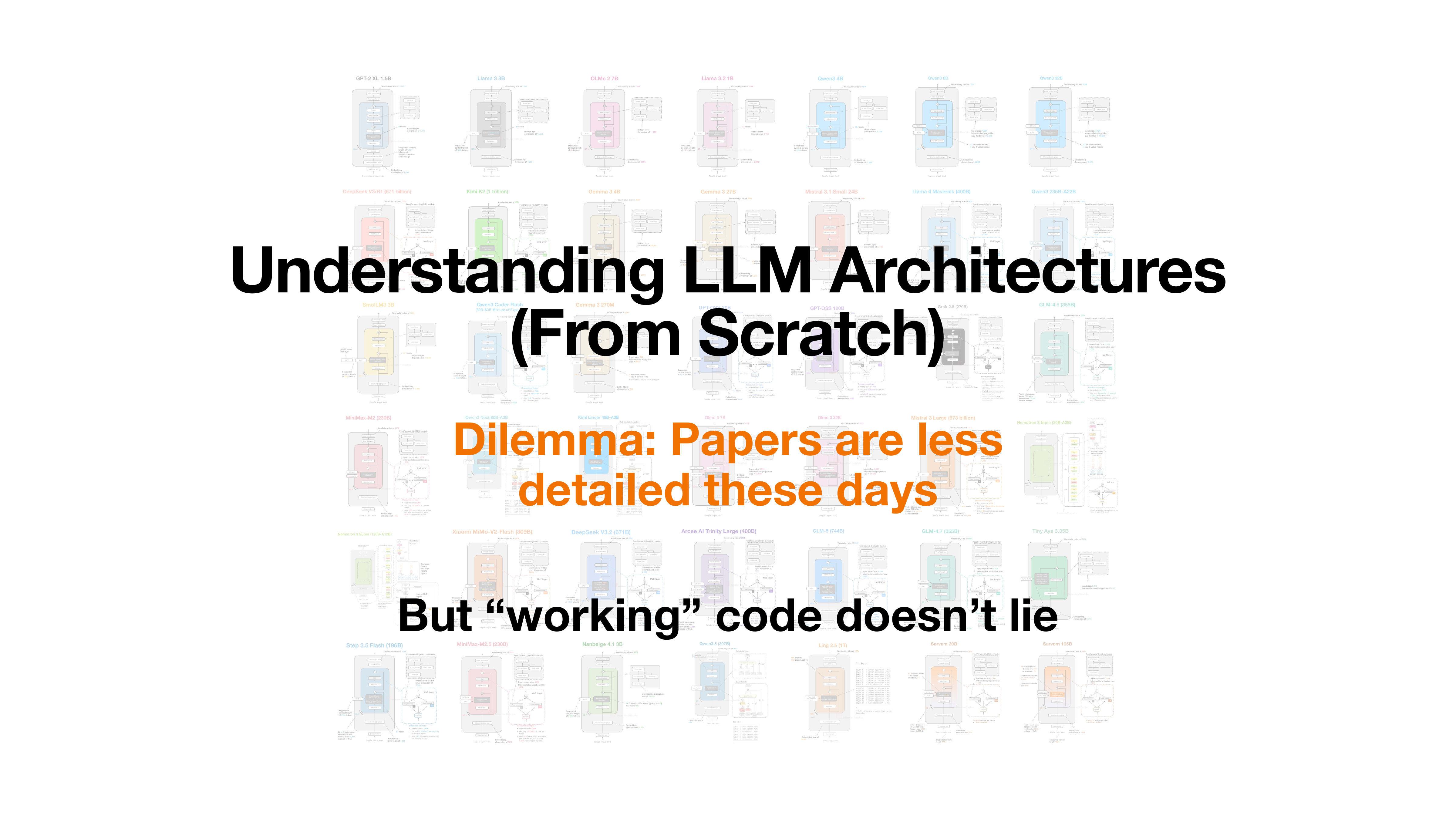
I should also say that this is mainly a workflow for open-weight models. It doesn’t really apply to models like ChatGPT, Claude, or Gemini, where the weights and details are proprietary.
Also, this is intentionally a fairly manual process. You could automate parts of it. But if the goal is to learn how these architectures work, then doing a few of these by hand is, in my opinion, still one of the best exercises.
We’re living through the period of time when we’ll learn if open models can keep up with closed labs. The obvious answer is that no, they won’t. This answer is a form of saying they won’t keep up in every area. This framing closes off a popular prediction where the open models completely catch up, as in all models saturate and open and closed models only become increasingly similar. In living through this, it’s evidently very unclear when the longer-term stable balance of capabilities will solidify.
This is a very complex dynamic, where the core point we monitor is a capability gap between models. At the same time, this gap is intertwined with evolving dynamics in the funding of open models, who builds open models, how techniques like distillation that enable fast-following translate through new application domains, potential regulation hampering the open-source AI ecosystem, and of course who actually uses open models.
The capabilities gap is one signal in a complex sea of forces, pushing supply and demand into different shapes. In many cases the demand — where obviously tons of individuals, organizations, and sovereigns want, or need, open models — is largely separated from supply. Supply is fully dictated by economics. The question of “which business strategies support releasing open models” is still at stake.
Interconnects AI is a reader-supported publication. To receive new posts and support my work, consider becoming a subscriber.
With this complexity, I wanted to distill my key beliefs down into a clear list. These are downstream of 10+ pieces I’ve written or recorded on open models this spring (which are linked throughout).
It’s surprising that the top closed models did not show a growing capability margin over open models, based on compute differences for training and research, especially in the second half of 2025 and through today.
Open model labs are technically very strong at keeping pace on well-established benchmarks. This will continue and reflects a balance of abundant talent and sufficient computing power.
Chinese open-weight labs focus slightly more on benchmark scores than comparable closed labs in the U.S. Distillation helps the Chinese LLM companies do so, but it’s not a panacea. Changes in the distillation dynamic (e.g. regulation) will not be a determining factor on the balance of capabilities. This increase in focus is a natural evolution of their incentives in keeping the narrative on keeping up with the frontier alive, which is crucial to fundraising and adoption.
To date, closed models tend to be more robust and generally useful than similarly scoring open models. Closed models have certain hard-to-measure qualities that are not well captured in current or past benchmarks. This will be key to enabling closed models to dominate in markets where an individual user constantly presents new challenges, i.e. supporting knowledge workers as a direct assistant.
The open vs. closed model race, as monitored through benchmarks, will largely be a game of economic staying power and fast-following, until the market structure constricts. I expect Chinese open-weight labs to face funding difficulties first, as soon as later this year. Funding difficulties will be seen in different capability trajectories 3-9 months later.
The RL dominated training era has increased the relevance of distribution to real-world use-cases as a key factor in continued capabilities improvements. These are tasks where users directly use tools like Claude Code or Codex to solve problems in their job with agents. This is the first clear technical area that closed labs can dominate open-weight models on capabilities, potentially leveraging online RL directly based on user feedback.
Open models will be increasingly adopted in repetitive automation tasks, as measured in the relative share of the API market, for repetitive tasks across the ecosystem. This takes the form of many new AI-native applications, business backend automation, etc. The success of this will drive more investment in domain-specific, efficient open models.
This is a complex picture, where the long-term trajectory is more of an economics question rather than an ability one. Many other outlets can paint a far more simplistic narrative that “China will assuredly catch us in AI” and get more distribution because it is a simple story. The reality is complex. Only real AI revenue begets more investment, eventually that’ll be linked to the ability to keep improving models at a rapid rate. Economic realities have not yet impacted scaling open models, as a general category.
This economic-focused angle relates to my positions on the open model ecosystem more broadly.
Recurring calls to ban certain types of open models will continue to come but are in practice impossible to implement. Training strong AI models (i.e. near but not at the frontier) is a relatively small cost compared to large-scale deployments. E.g. if the U.S. bans open models over a certain compute threshold, another sovereign entity will eventually train them and release them publicly, with the models entering the U.S. market with less oversight.
The second derivative of influence on open models has shifted, and the U.S. will slowly regain ground in adoption metrics of open models starting in early 2027 (it takes a long time for China’s velocity to slow, then flip). Examples include Google’s Gemma 4 (a wild success), Nvidia’s Nemotron, and Arcee AI.
As ever-stronger closed models are built, previewed, and released, there will be more safety-shocks saying that open-weight versions of the strongest AI models never can be allowed to exist, similar to reactions to Claude Mythos. These can spur burdensome regulation on open models.
With the above, there will also be increased long-term interest in open models, as sovereign entities and existing power structures realize the coming, super powerful AI tools cannot land in the hands of only one or a few companies. These entities will see open models as a different governance paradigm.
New funding structures for open models will emerge, as many stakeholders realize dependencies on single, for-profit companies for access to intelligence are unreliable.
Local agents, OpenClaw, and other personal agents represent a large, to date, mostly ignored market for open model usage. It is a sort of dark matter, with pervasive, massive potential for influence on the balance of open-to-closed models.
A single word governs this post and is intentionally repeated — complex.
This complex reality has been driving me to think more deeply about how to clearly describe the open model gap, and why I can hold it in my head that I expect American closed labs to clearly draw ahead, despite the fairly unequivocal evidence in support of the capabilities of recent open-weight models. More on the nuance in the open-closed gap in another piece coming soon, so please subscribe!
Let me know any positions that I missed.
For every dollar spent on software, six are spent on services. Why? Because buying enterprise software is easy. Implementing it is hard, and still leans heavily on labour. Across the top 10 software ecosystems (ServiceNow, Salesforce, SAP, AWS, and others), 9 million implementation consultants represent more than $500 billion in annual labour spend, still growing 10%+ a year. It’s one of the largest markets in technology, and one of the least disrupted.
Enterprise platforms have thousands of components that change daily. A single deployment can span hundreds of requirements, dozens of stakeholders, and months of back-and-forth between what a business needs and what the system can actually do. Today, consultants hold all of this together through experience and pattern recognition. But they forget context between meetings. They miss dependencies across systems. They can’t track thousands of platform updates simultaneously. Unlike LLMs, their context windows are limited by biology.
Auctor is the autopilot for software implementation, from the moment a customer requirement is captured all the way through to delivery. It brings together the requirements, decisions, and context that typically live across meetings, documents, and dozens of disconnected systems, and translates them directly into the outputs needed to move a project forward. What used to take teams weeks of scoping now gets done in a single sitting.
We first partnered with Auctor at the Seed, shortly after the team graduated from YC. At Sequoia, each year we select a handful of portfolio companies and take their founders to meet executives at some of the most important technology companies in Silicon Valley. For an hour, these leaders effectively join the team, helping us and the founders think through strategy, positioning, and go-to-market. In our very first meeting with the C-suite of a major enterprise platform, the executives asked for a pilot halfway through the conversation, before we’d even demoed the product.
What gave us conviction beyond the market was the team. This is a category where speed of execution determines the winner given the first mover advantage. Will, Sky, and Matt are the hardest-charging, fastest-moving team we’ve met in this space. They shipped their platform and landed their first major enterprise contract within months of graduating YC. They’ve set up shop in New York and are pulling in talent the way only a team with this much momentum can.
We’re leading Auctor’s Series A and couldn’t be more excited to partner with Will and the team to bring software implementation into the age of AI.
The post Partnering with Auctor appeared first on Sequoia Capital.
